Cross-movie prediction of individualized functional topography
- Center for Cognitive Neuroscience, Dartmouth College, United States
- Princeton Neuroscience Institute, Princeton University, United States
- Department of Medical and Surgical Sciences (DIMEC), University of Bologna, Italy
- IRCCS, Istituto delle Scienze Neurologiche di Bologna, Italy
Figures
Figure 1 with 1 supplement
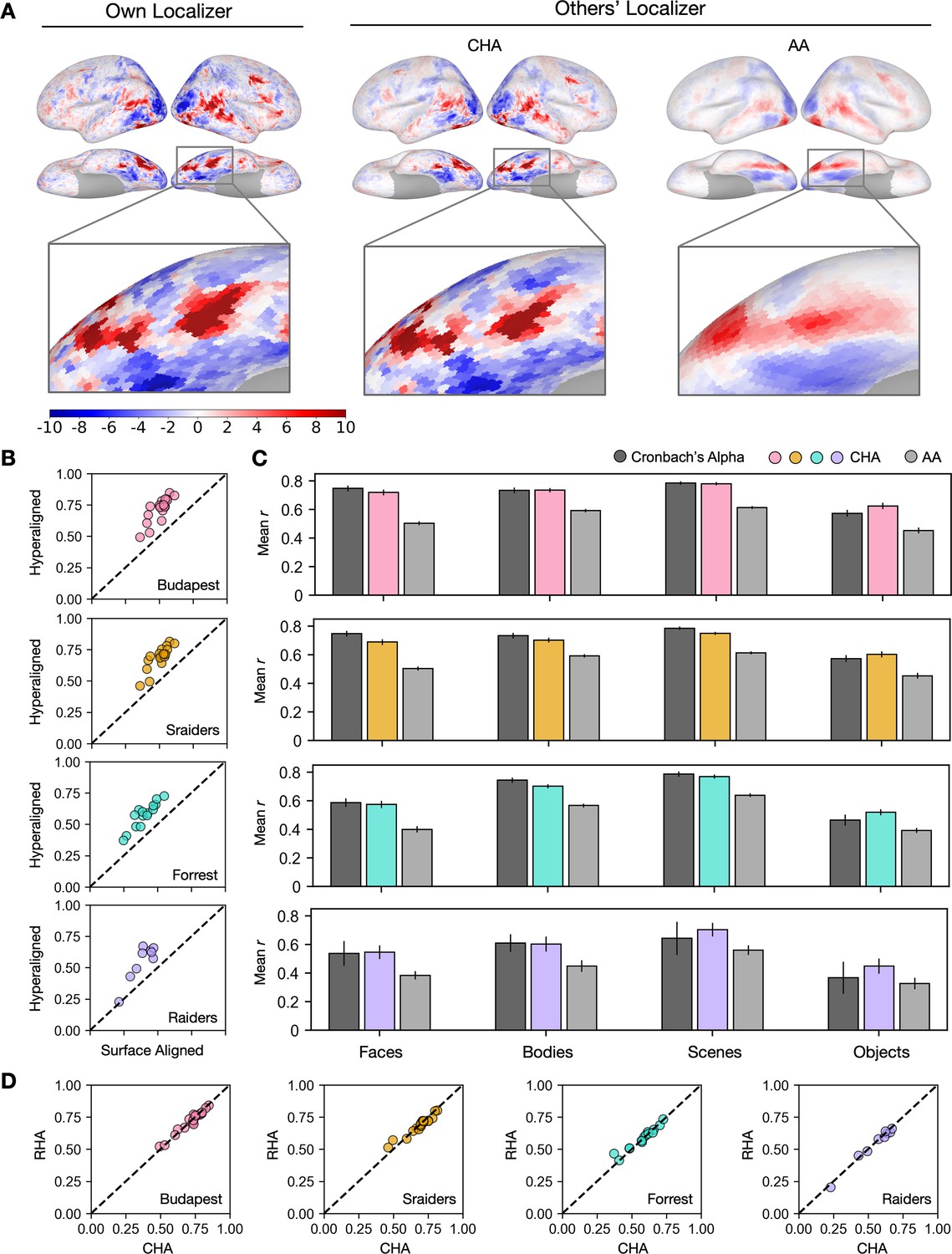
Predicting individual category-selective topographies using connectivity hyperalignment (CHA).
(A) Face-selective topographies (faces-vs-all) and zoomed-in views of an example participant estimated from this participant’s own localizer (Own Localizer), and other participants’ localizers using CHA, and surface anatomical alignment (AA). (B) Scatter plots display the Pearson correlation coefficients between estimated face-selective topographies based on own localizer data and other participants’ localizer data in individual participants in four different datasets. The y-axis corresponds to correlations between each target participant’s own localizer-based face-selective topographies and face-selective topographies estimated from other participants using CHA. The x-axis corresponds to correlations between each target participant’s own localizer-based face-selective topographies and face-selective topographies estimated from other participants with surface-based anatomical alignment. (C) Bar plots show the mean correlations across participants in four datasets (Budapest & Sraiders: n = 20; Forrest: n = 15; Raiders: n = 9. Same sample sizes in other figures for each dataset unless noted.) and for all four category-selective topographies. Black bars stand for the mean Cronbach’s alphas across participants. Error bars indicate ±1 standard error of the mean. Category topographies were defined based on contrasts between the target category and all other categories. (D) Scatter plots of Pearson correlation coefficients using CHA and response hyperalignment (RHA) for individual participants within four different datasets for the face-selective topography. Values on the y-axis stand for correlations between each target participant’s own localizer-based topographies and topographies estimated from other participants in the same dataset using RHA. Values on the x-axis stand for correlations between each target participant’s own localizer-based topographies and topographies estimated from other participants in the same dataset using CHA.
Figure 1—figure supplement 1
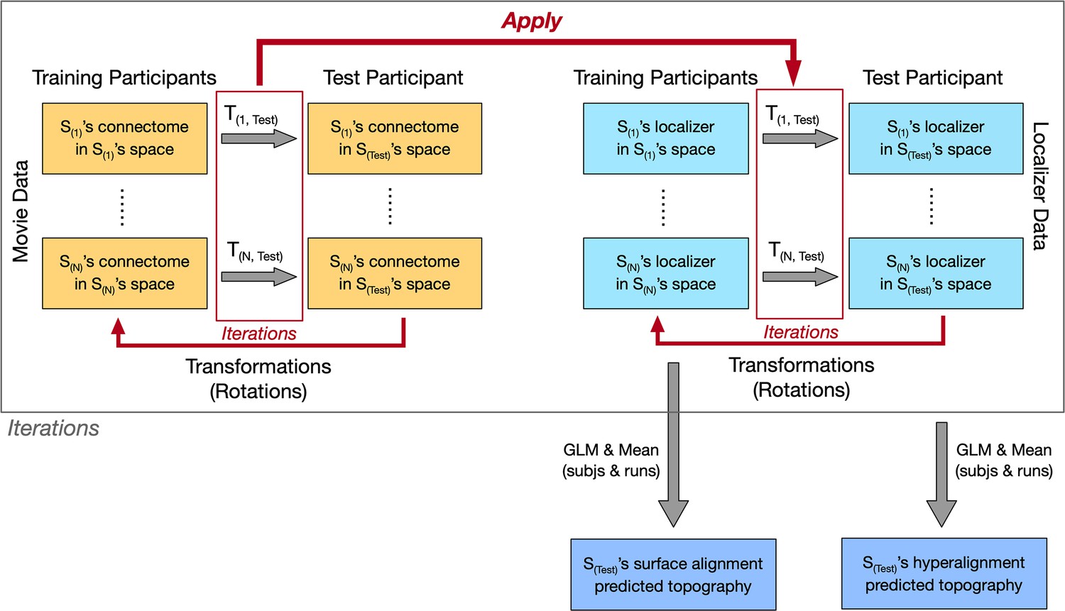
Schematic data analysis procedures.
In the enhanced connectivity hyperalignment (CHA) analysis, transformation matrices derived from projecting connectome based on the movie data in each training participant’s cortical space to the target participant’s space were applied to each training participant’s localizer runs. These steps were iterated six times, and in each step, the connectome and the localizer data were both updated. The original localizer runs were used to calculate category-selective topographies for each training participant and averaged across runs and participants to obtain the surface alignment predicted topography for the target participant. The localizer runs hyperaligned after all iteration steps were used to obtain CHA predicted topographies with similar procedures. Outside of this loop, each target participant’ own original localizer runs were used to obtain this participant’s own localizer estimated topographies.
Figure 2 with 2 supplements
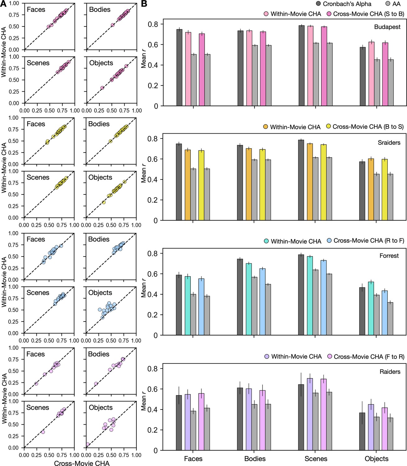
Predicting category-selective topographies using connectivity profiles across movies.
(A) Scatter plots of Pearson correlation coefficients for individual participants in four different datasets and for four categories. Values on the y-axis stand for correlations between each target participant’s own localizer-based topographies and topographies estimated from other participants in the same movie using connectivity hyperalignment (CHA). Values on the x-axis stand for correlations between each target participant’s own localizer-based topographies and topographies estimated from participants in another dataset based on cross-movie CHA. (B) Bar plots display the mean Pearson correlation coefficients (r) and Cronbach’s alphas across participants in all four datasets for all four categories. Error bars stand for ±1 standard error of the mean. S to B: Sraiders to Budapest, B to S: Budapest to Sraiders, R to F: Raiders to Forrest, F to R: Forrest to Raiders.
Figure 2—figure supplement 1
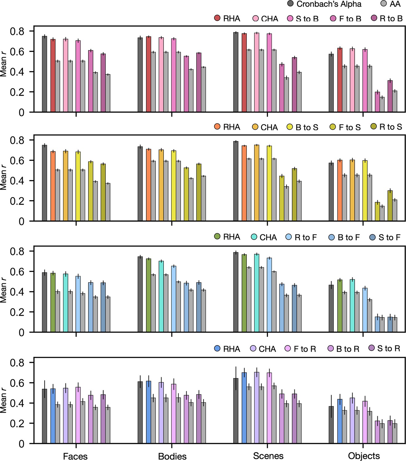
Connectivity hyperalignment (CHA) predictions.
Bar plots display the mean Pearson correlation coefficients (r) and Cronbach’s alphas across participants in all four datasets for all four categories. Error bars stand for ±1 standard error of the mean. The abbreviations are the same in all figures, including this one. S to B: Sraiders to Budapest, F to B: Forrest to Budapest, R to B: Raiders to Budapest, B to S: Budapest to Sraiders, F to S: Forrest to Sraiders, R to S: Raiders to Sraiders, R to F: Raiders to Forrest, B to F: Budapest to Forrest, S to F: Sraiders to Forrest, F to R: Forrest to Raiders, B to R: Budapest to Raiders, S to R: Sraiders to Raiders.
Figure 2—figure supplement 2
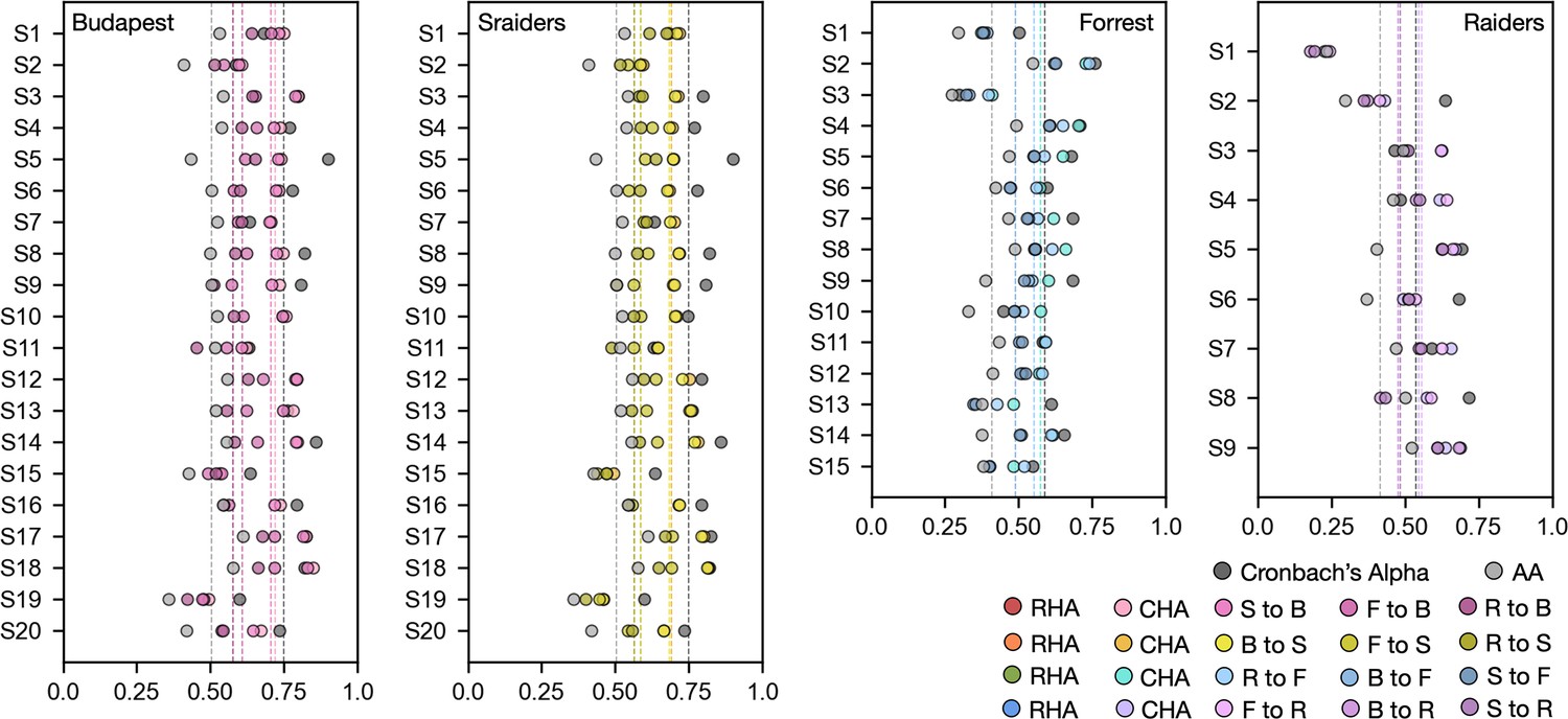
Prediction performances for each individual participant.
Prediction performance (Pearson r) for the face-selective topography for each individual participant using response hyperalignment (RHA), connectivity hyperalignment (CHA), cross-movie CHA, and surface alignment (AA) in all four datasets. Black dots stand for individual participants’ Cronbach’s alphas of their own face-selective topographies across localizer runs. Dashed lines are the mean values across participants. S to B: Sraiders to Budapest, F to B: Forrest to Budapest, R to B: Raiders to Budapest, B to S: Budapest to Sraiders, F to S: Forrest to Sraiders, R to S: Raiders to Sraiders, R to F: Raiders to Forrest, B to F: Budapest to Forrest, S to F: Sraiders to Forrest, F to R: Forrest to Raiders, B to R: Budapest to Raiders, S to R: Sraiders to Raiders.
Figure 3 with 2 supplements
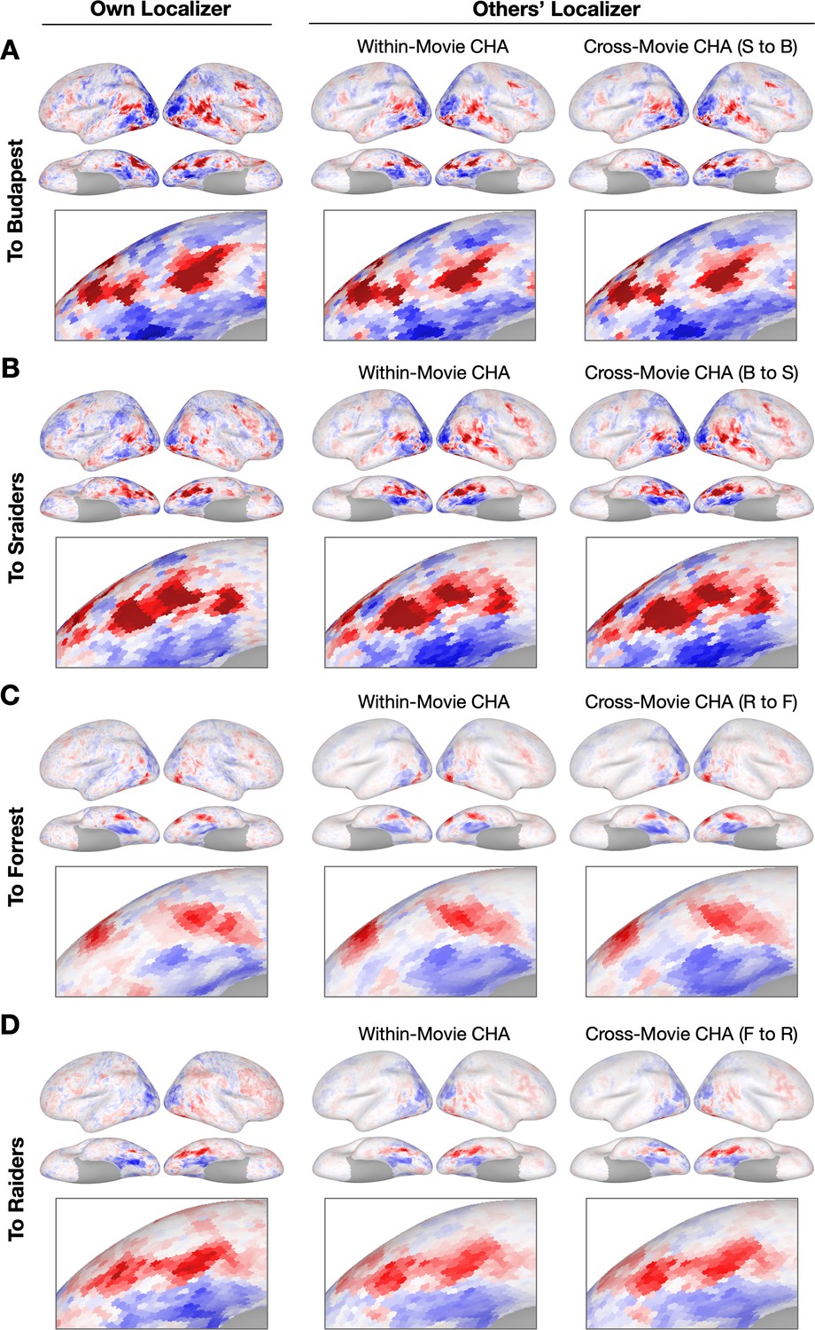
Sample contrast maps and enlarged views of the ventral temporal cortex.
Contrast maps for face-selective topographies (faces-vs-all) and their zoomed-in views of the ventral temporal cortex were plotted in four sample participants in (A) Budapest, (B) Sraiders, (C) Forrest, and (D) Raiders. In all four subplots, in the left-most panel, faces-vs-all maps were plotted on the sample participants’ own cortical surfaces. The next two columns display maps estimated from other participants’ data. In the right two columns, the first column presents predicted face-selective topographies from participants in the same dataset using connectivity hyperalignment (CHA). The next column presents face-selective topographies from participants in another dataset (cross-movie CHA). The zoomed-in panels are displayed accordingly with the whole-brain map. The color bar is the same as that in Figure 1. S to B: Sraiders to Budapest, B to S: Budapest to Sraiders, R to F: Raiders to Forrest, F to R: Forrest to Raiders.
Figure 3—figure supplement 1
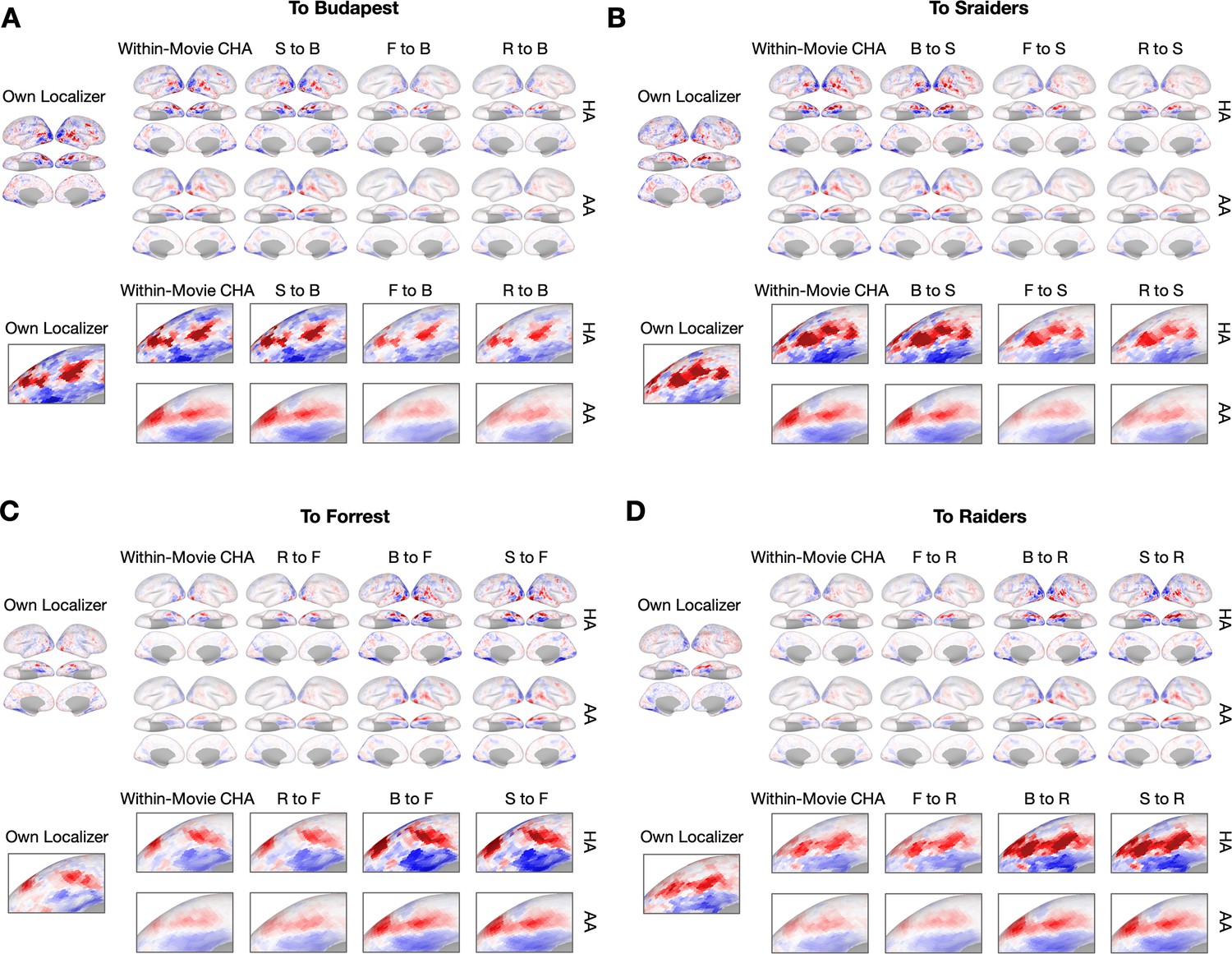
Sample contrast maps and enlarged views of the ventral temporal cortex.
Contrast maps for face-selective topographies (faces-vs-all) and their enlarged views of the ventral temporal cortex were plotted in sample participants in (A) Budapest, (B) Sraiders, (C) Forrest, and (D) Raiders. In all five subplots for the whole-brain maps, the faces-vs-all maps were plotted on the sample participants’ own cortical surfaces (left single panel). The second column presents predicted face-selective topographies from participants in the same dataset using connectivity hyperalignment (top) and surface alignment (bottom). The next three columns present face-selective topographies from participants in another dataset with the same (second column) and a different type (the last two columns) of localizers. In the four right columns, the top row presents the map using hyperalignment (HA), and the bottom row presents the map using surface alignment (AA). The enlarged panels were displayed accordingly with the whole-brain map. The color bar was the same as that in Figure 1.
Figure 3—figure supplement 2
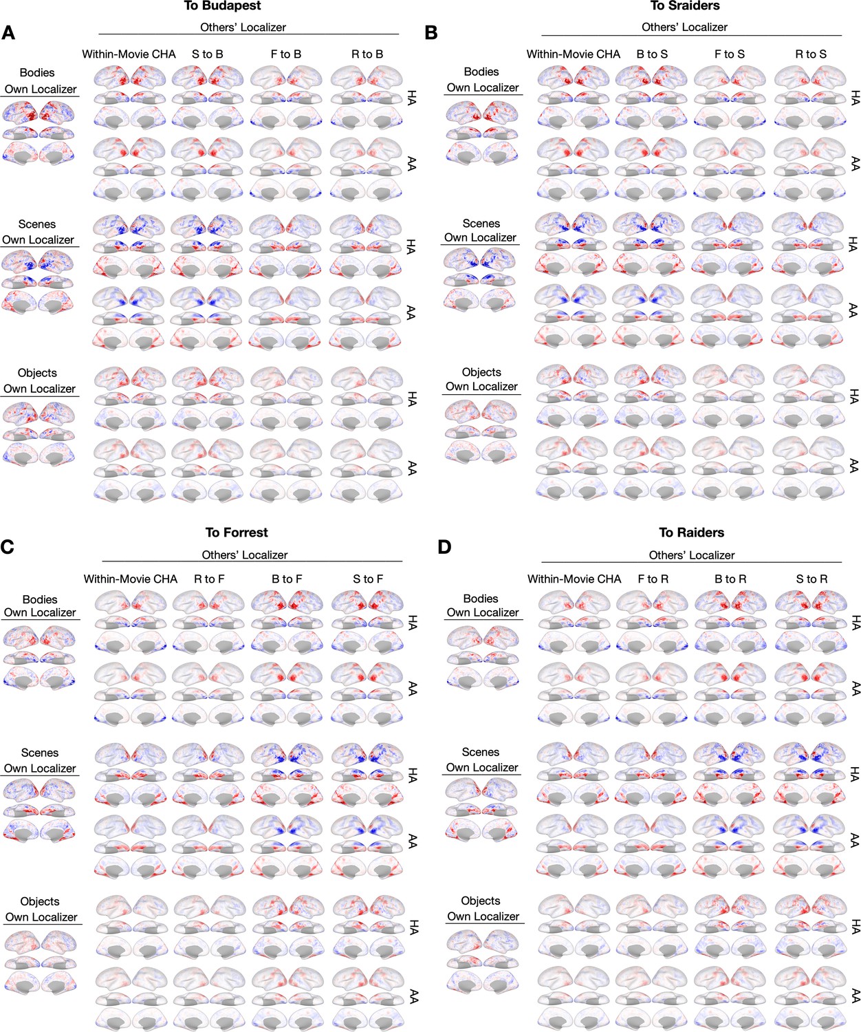
Sample contrast maps of body-, scene-, and object-selective topographies.
Contrast maps of the other three categories were plotted in participants in (A) Budapest, (B) Sraiders, (C) Forrest, and (D) Raiders. In all five subplots for the whole-brain maps, the maps estimated from their own localizer runs were plotted on the sample participant (left single panel). The other columns present predicted topographies from participants in the same dataset using connectivity hyperalignment (top) and surface alignment (bottom).
Figure 4 with 10 supplements
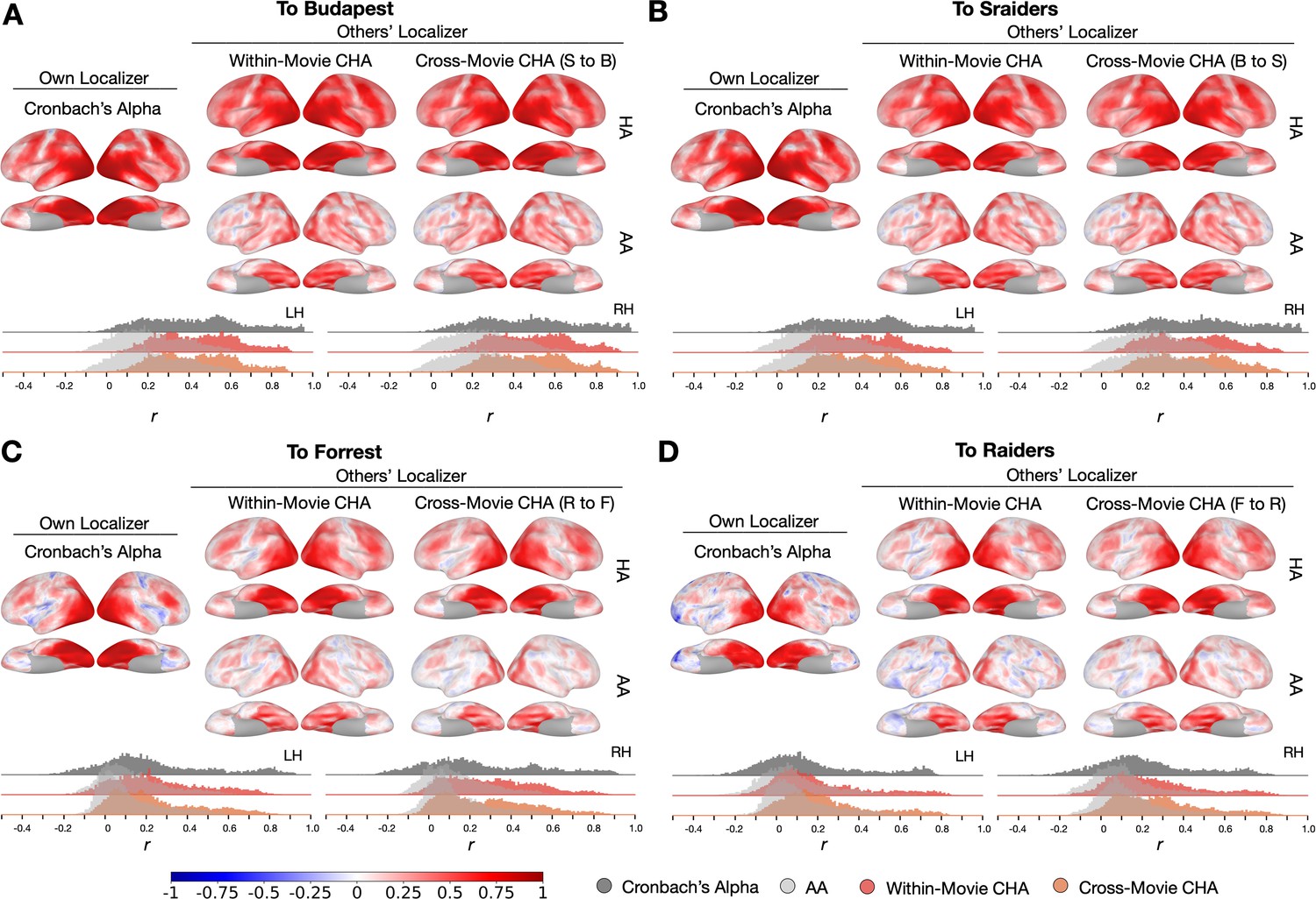
Searchlight analysis of Cronbach’s alphas and prediction performances.
(A, B, C, and D) The left-most column presents Cronbach’s alphas of the own-localizer-based face-selective topographies in each dataset using a searchlight analysis (15 mm radius). The next two columns present local correlations (correlation maps) using the searchlight analysis between face-selective maps estimated from participants’ own localizers and from other participants based on within-movie and between-movie connectivity hyperalignment (CHA) (hyperalignment [HA], top row) and surface alignment (AA, bottom row). Histogram plots present Cronbach’s alphas (dark gray) and coefficients for the correlation maps above (estimated with CHA in color, with AA in light gray). The left and right hemisphere histograms were plotted separately. B to S: Budapest to Sraiders, S to B: Sraiders to Budapest, R to F: Raiders to Forrest, F to R: Forrest to Raiders.
Figure 4—figure supplement 1
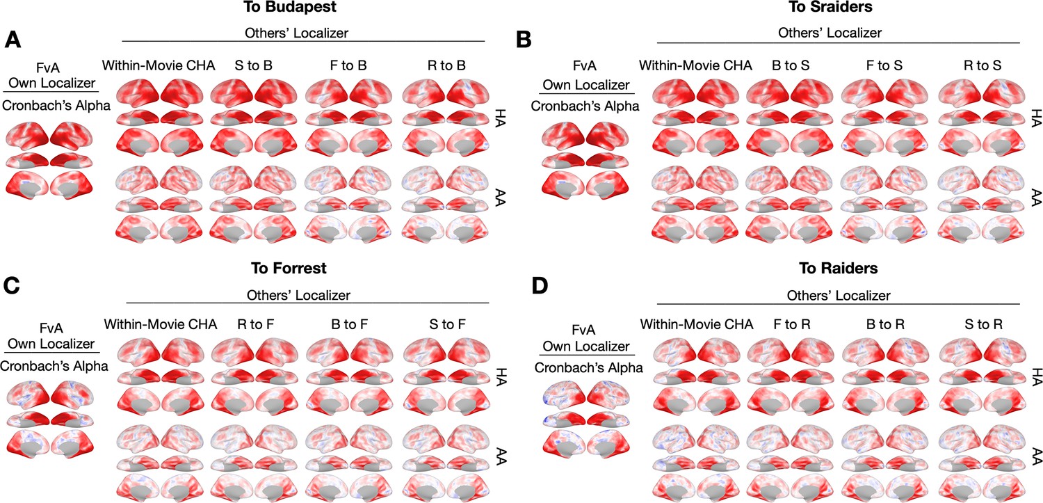
Searchlight correlations.
(A, B, C, and D) The left-most column shows the Cronbach’s alphas of the own localizer-based face-selective topographies in each dataset using a searchlight analysis (15 mm radius). The next four columns show local correlations (correlation maps) using the searchlight analysis between the face-selective maps estimated from other participants based on within-movie (second column, top row) and between-movie (the next three columns, top row) connectivity hyperalignment (CHA) and surface alignment (AA, bottom row).
Figure 4—figure supplement 2
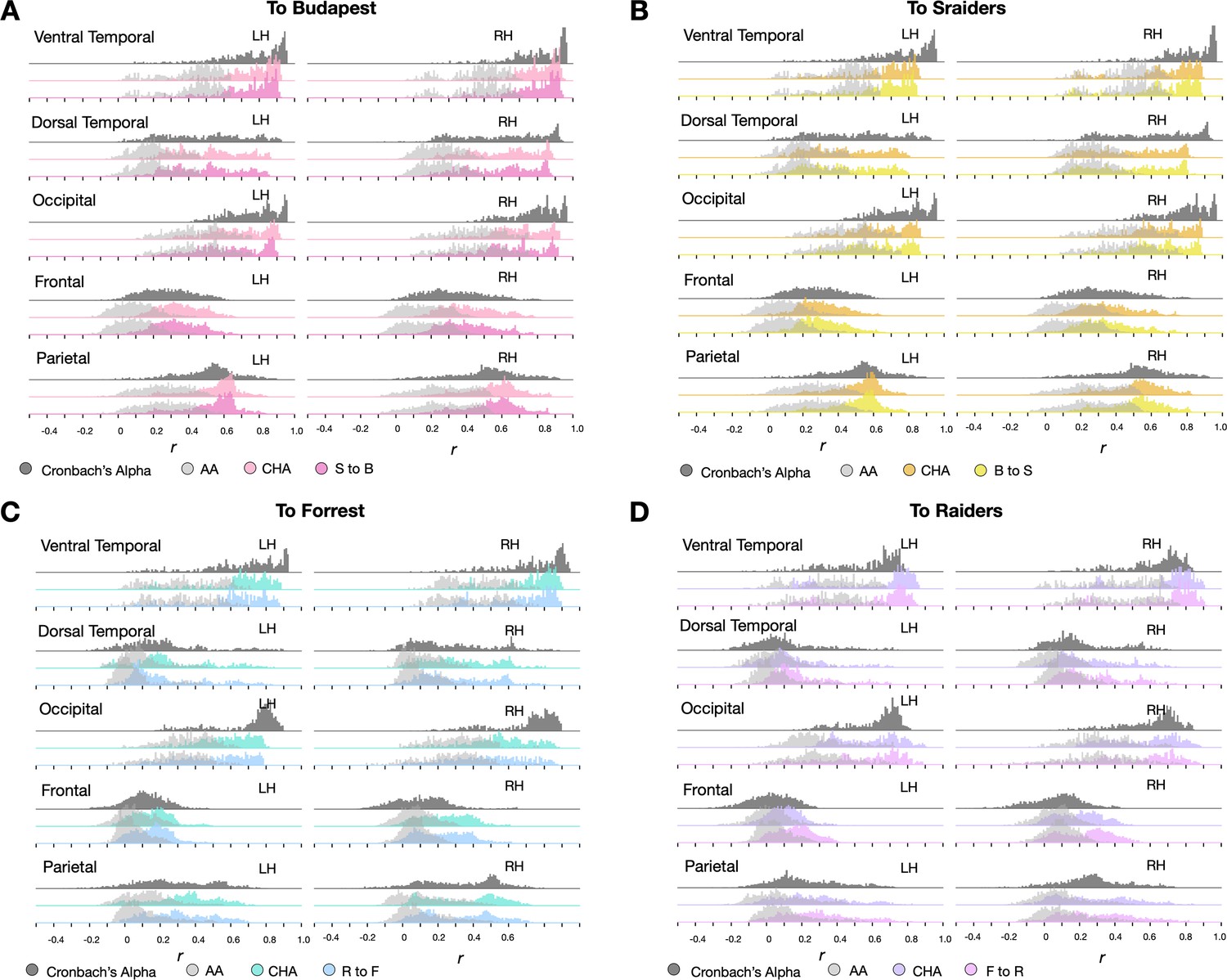
Distribution of correlation coefficients in major cortices.
Histogram plots of local Cronbach’s alphas (dark gray) and local correlation coefficients between face-selective topographies estimated from own and others’ localizers across the cortex (hyperalignment [HA] in color, light gray for surface alignment [AA]) in major cortices (ventral temporal, dorsal temporal, occipital, frontal, and parietal) in the four datasets (see Figure 4 for the whole-brain maps and distributions). The left and right hemisphere histograms were plotted separately in each cortical parcel.
Figure 4—figure supplement 3
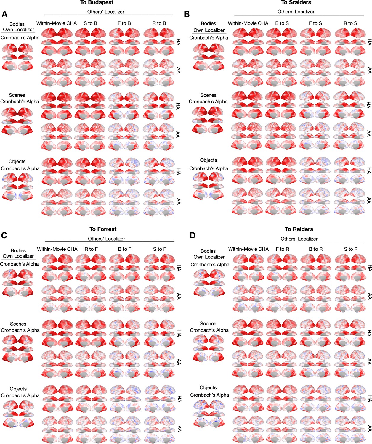
Searchlight analysis results for other categories.
(A, B, C, and D) The left-most column shows the Cronbach’s alphas of the own localizer-based topographies in each dataset using a searchlight analysis (15 mm radius). The next four columns show local correlations (correlation maps) using the searchlight analysis between the category-selective maps estimated from other participants based on within-movie (second column, top row) and between-movie (the next three columns, top row) connectivity hyperalignment (CHA) and surface alignment (AA, bottom row).
Figure 4—figure supplement 4
Advanced connectivity hyperalignment (CHA) improved prediction performances.
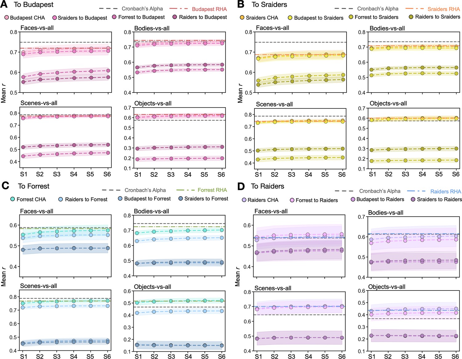
(A) In each subplot, each line with dots showed the improvement of the mean correlation across participants between the category-selective maps estimated from each participant’s own localizer runs and those estimated from participants’ data in other datasets from step 1 to step 6 using our new advanced iterative CHA algorithm. Horizontal dotted lines are the mean Cronbach’s alphas (gray) and the mean performance using response hyperalignment (RHA) (colored). (B, C, and D) had the same layout as A with participants in Sraiders, Forrest, and Raiders dataset as the prediction target.
Figure 4—figure supplement 5
Prediction performance changing with number of runs and participants.
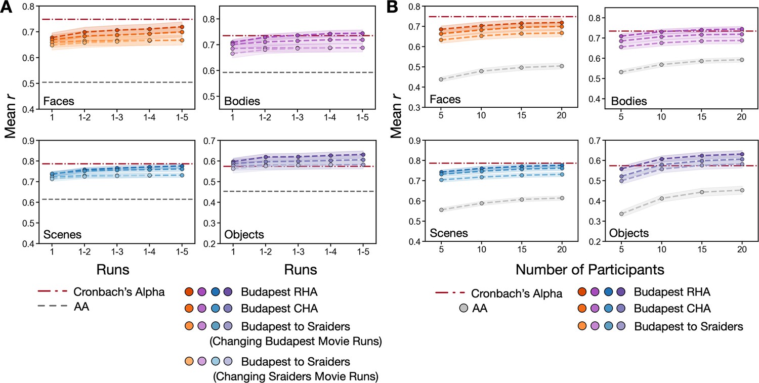
(A) In each subplot, each line with dots showed the improvement of the mean correlation across participants between the category-selective maps (faces, bodies, scenes, and objects) estimated from each participant’s own localizer runs and those estimated from other participants’ data using the 1, 1–2, 1–3, 1–4, and all five runs of the Budapest movie or all four runs of the Sraiders movie. The length of each movie-viewing run in the Budapest dataset is 598 s, 498 s, 535 s, 618 s, and 803 s accordingly, and 840 s for each of the four runs in the Sraiders dataset. Horizontal dotted lines are the mean Cronbach’s alphas (red) and the mean performance based on surface alignment (gray). (B) In each subplot, each line with dots showed the improvement of the mean correlation across participants between the category-selective maps (faces, bodies, scenes, and objects) estimated from each participant’s own localizer runs and those estimated from other participants’ data using 5, 10, 15, or all 20 participants in the Budapest dataset. Horizontal dotted lines are the mean Cronbach’s alphas (red) and gray lines with dots showing the mean performance based on surface alignment.
Figure 4—figure supplement 6
Predictions based on the 1-step and the 2-step methods.
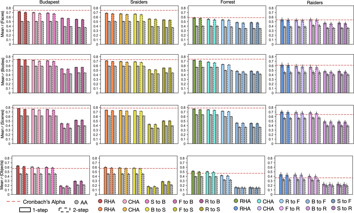
Bar plots display the mean Pearson correlation coefficients (r) and Cronbach’s alphas across participants in all four datasets for all four categories. Bars with solid outlines stand for results based on the 1-step method, and bars with dashed outlines are based on the 2-step method. Error bars stand for ±1 standard error of the mean.
Figure 4—figure supplement 7
Comparing prediction performance between projecting time series and projecting contrast maps to the target participant.
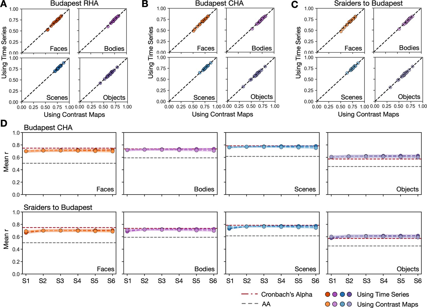
(A, B, and C) Scatter plots of Pearson correlation coefficients with Budapest dataset, using response hyperalignment (RHA), connectivity hyperalignment (CHA), and cross-movie from Sraiders to Budapest for individual participants for the face, body, scene, and object-selective topographies. Values on the y-axis stand for correlations between each target participant’s own localizer-based topographies and topographies estimated from other participants when transformation matrices were applied to the localizer time series. Values on the x-axis stand for correlations between each target participant’s own localizer-based topographies and topographies estimated from other participants when transformation matrices were applied directly to contrast maps. (D) In each subplot, each line with dots showed the mean correlation across participants between the category-selective maps estimated from each participant’s own localizer runs and those estimated from participants’ data in other datasets from step 1 to step 6 using the new advanced iterative CHA algorithm. Darker shades stand for the performance when transformation matrices were applied to localizer time series, and lighter shades stand for the mean performance when transformation matrices were applied directly to contrast maps. Horizontal dotted lines are the mean Cronbach’s alphas (red) and the mean performance using only surface alignment (gray).
Figure 4—figure supplement 8

Prediction performance using participants with similar connectivity profiles.
Bar plots display the mean Pearson correlation coefficients (r) across participants using all or part of the training participants for face-selective topography using connectivity hyperalignment (CHA) with the Budapest dataset. Participants were divided based on their connectivity profile similarities to the target participant and were measured using a 10 mm searchlight in the right ventral temporal cortex that was roughly at the location of the posterior fusiform face area (rpFFA). Bars in color are based on CHA, and bars in gray are based on surface alignment. Error bars stand for ±1 standard error of the mean.
Figure 4—figure supplement 9
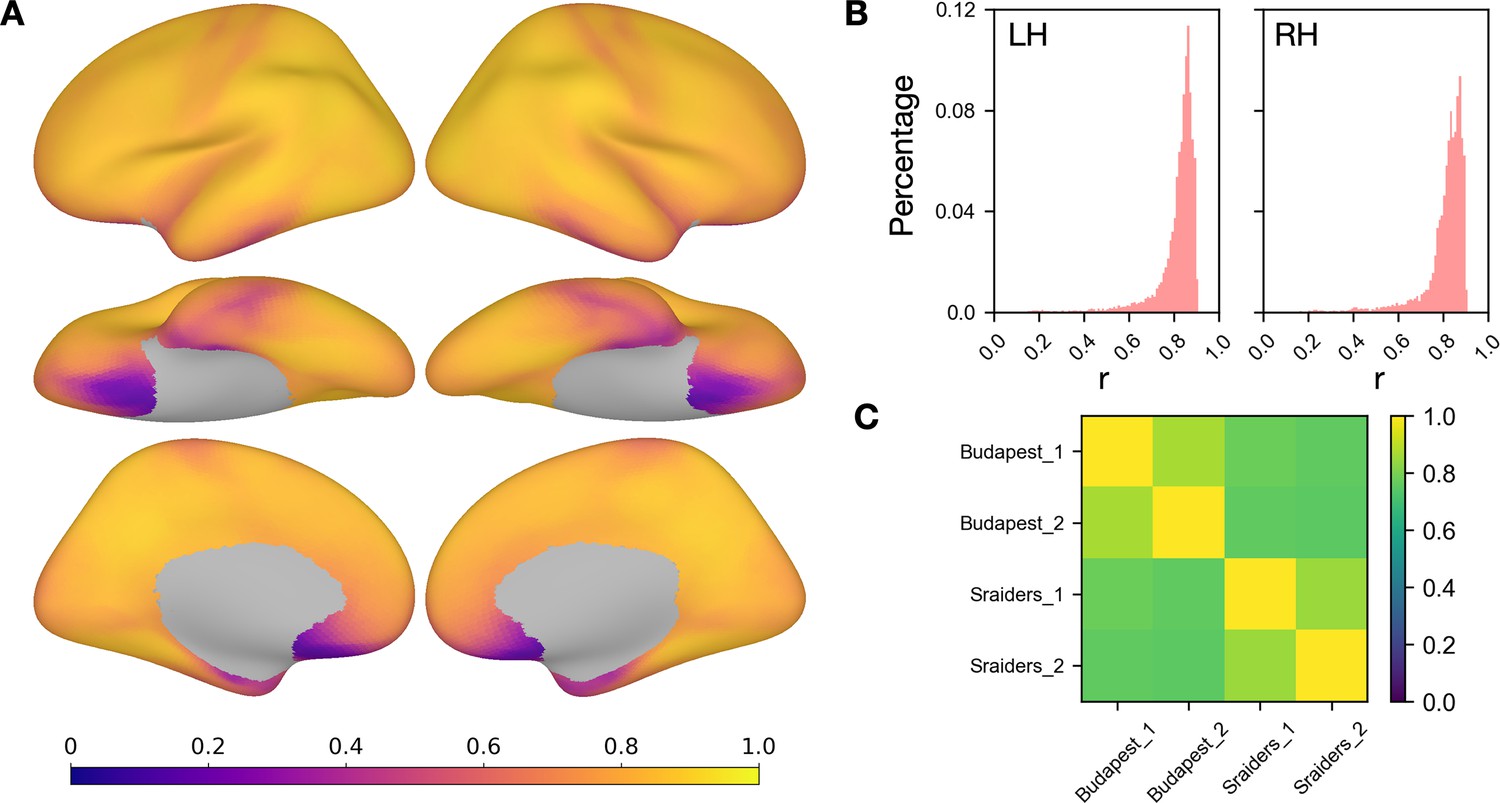
Similarities between fine-grained connectivities in two different movie-viewing tasks.
(A) For each participant in the Budapest and the Sraiders dataset, connectomes that described the connectivity between each target in the searchlight and each vertex on the cortex were calculated for each dataset and correlated across the two datasets. This whole-brain map shows the mean correlations across participants. (B) Histogram plots of the correlation coefficients in A in the left and the right hemisphere. (C) The two datasets were split into two halves, and similarities of the fine-grained connectivity between the two halves within and across the two movies were calculated following the same procedures above. This plot shows the mean correlations across participants and searchlights.
Figure 4—figure supplement 10
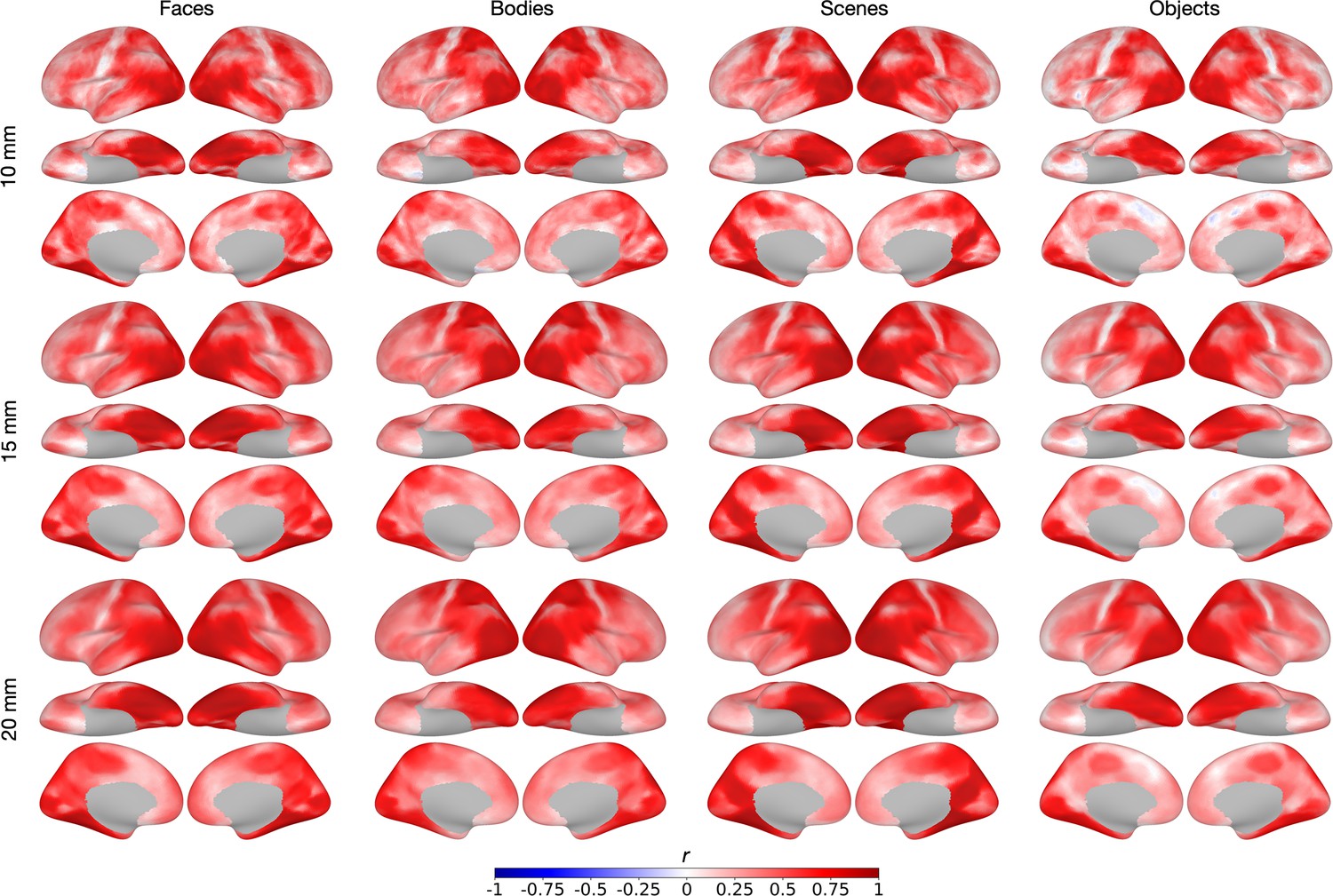
Searchlight correlations with different searchlight sizes.
Each set of brain maps shows the averaged local correlations between the category-selective map (column) estimated from other participants in the Budapest dataset based on enhanced connectivity hyperalignment (CHA) and the map estimated from their own localizers using a specific size of searchlight (row). Local correlations remained relatively similar across different searchlight sizes for all categories.
Author response image 1

Additional files
Download links
A two-part list of links to download the article, or parts of the article, in various formats.
Downloads (link to download the article as PDF)
Open citations (links to open the citations from this article in various online reference manager services)
Cite this article (links to download the citations from this article in formats compatible with various reference manager tools)
Cross-movie prediction of individualized functional topography
eLife 12:e86037.
https://doi.org/10.7554/eLife.86037


