An open-source platform for head-fixed operant and consummatory behavior
- Center for the Neurobiology of Addiction, Pain, and Emotion, Department of Anesthesiology and Pain Medicine, Department of Pharmacology, University of Washington, United States
- Department of Psychology, University of Illinois at Chicago, United States
- Graduate Program in Neuroscience, University of Illinois at Chicago, United States
Figures
Figure 1 with 1 supplement
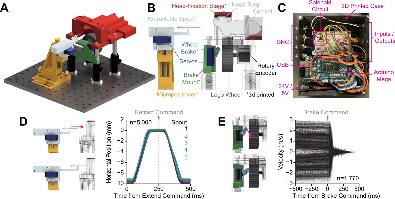
OHRBETS (Open-Source Head-fixed Rodent Behavioral Experimental Training System) operant conditioning.
Overview of functionality for operant conditioning (additional, optional multi-solution functionality illustrated in Figure 5). (A) 3D rendering of OHRBETS. (B) Cartoon depicting the critical components of our system (* indicates 3D printed components). (C) Image of the Arduino-based microprocessor and custom enclosure used for controlling hardware and recording events. (D) Validation of our 3D printed retractable spout powered by a low-cost micro servo. Left: 3D rendering of the linear travel of the spout; right: horizontal position of the spout tip determined using DeepLabCut over time during 1000 extension/retractions with five unique retractable spout units. (E) Validation of our 3D printed wheel brake powered by a low-cost micro servo. 3D rendering of the rotational travel of the wheel brake (left); binned rotational velocity of the wheel produced by manual rotation before and after the brake is engaged (right).
Figure 1—figure supplement 1
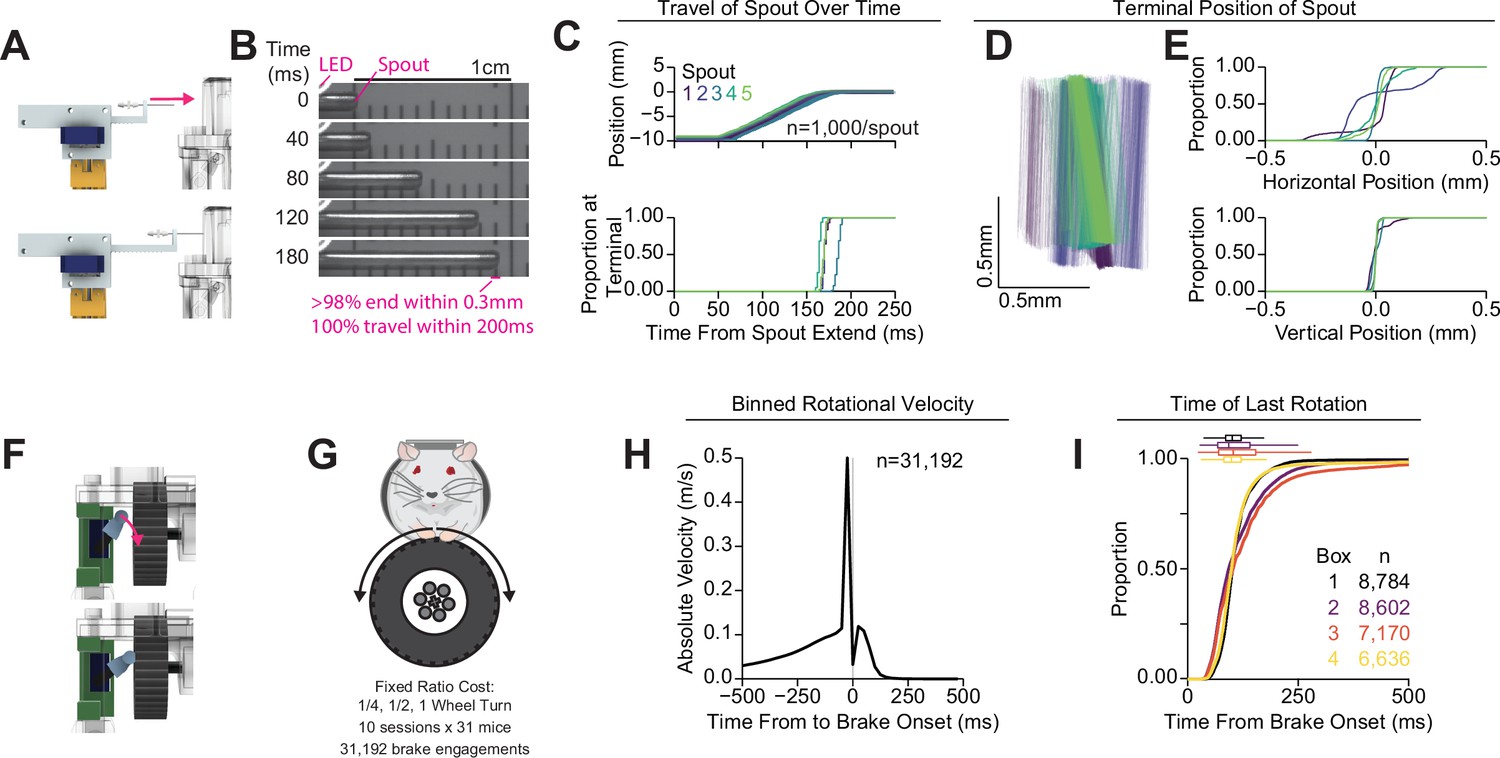
Validation of retractable spout and wheel brake.
(A) Cartoon of validation of the retractable spout. (B) Representative still frames from video data recording the position of the spout during 1000 extension/retractions in five different retractable spout assemblies. An LED was used to indicate the onset of the extension command (top left of frame). (C) Horizontal position of the spout during extension (top) and cumulative distribution of latencies to reach 98% of the final spout position (bottom). (D) Terminal position of the spout on all recorded extensions drawn from tracking the top and bottom corners of the spout (color indicates the identity of the spout assembly, lines represent the tip of the spout in 2D space for each trial). (E) Cumulative distribution of the horizontal (top) and vertical (bottom) position of the spout at the terminal location relative to the mean position at the terminal location, indicating incredibly consistent vertical positioning of the spout and highly consistent horizontal positioning of the spout. (F) Cartoon of validation of the wheel brake. (G) Cartoon indicating that data from fixed-ratio self-administration of 10% sucrose was used for (H–I) (n=31,192 wheel brake engagements). (H) Mean absolute velocity during 25 ms bins (SEM is not visible behind the line). (I) Cumulative distribution of the time of last detected rotation across every trial for each of the four behavioral setups (box and whisker plots indicate the median and interquartile range).
Figure 2 with 4 supplements
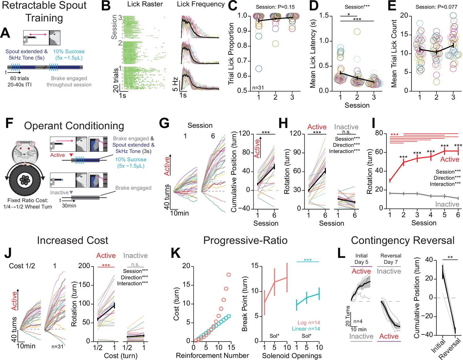
Mice rapidly learn head-fixed operant conditioning for sucrose and display operant behaviors established in freely moving experiments.
(A) Cartoon depicting the task design for retractable spout training. (B) Licking behavior throughout retractable spout training; lick raster for a representative mouse with each lick represented as a tick (left); mean binned frequency of licks (right). (C–E) Summary of behavior throughout retractable spout training: proportion of trials with at least one lick (C; one-way repeated measures [RM] ANOVA, session effect, F(2, 60)=1.98, p=0.15); mean latency from spout extension command to first lick on trials with a lick (D; one-way RM ANOVA, session effect, F(2, 60)=11.48, ***p=6.01e-5; Tukey honest significant difference [HSD] post hoc, *p<0.05, ***p<0.001); mean number of licks within each 5 s access period (E; one-way RM ANOVA, session effect, F(2, 60)=2.68, p=0.077). (F) Cartoon depicting the task design for operant conditioning. (G) Cumulative position of the wheel throughout the session (left) and at the conclusion of the session (right) on the first and sixth session of training (positive direction indicates rotation in the active direction; Welch two-sample t-test [paired, two-sided], t(30)=2.68, ***p=5.8E-9). (H, I) Total rotation of the wheel throughout a session broken down based on direction on the first and sixth session of training (H; two-way RM ANOVA, session effect, F(1, 30)=70.15, ***p=2.39e-9, rotation direction effect, F(1,30)=71.48, ***p=1.96e-9, session × rotation direction interaction, F(1,30)=64.48, ***p=5.8e-9, HSD post hoc, ***p<0.001) and across training sessions (I; two-way RM ANOVA, session effect, F(5, 150)=22.25, ***p=1.22e-16, rotation direction effect, F(1,30),=78.16, ***p=7.43e-10, session × rotation direction interaction, F(5,150)=23.54, ***p=2.03e-17, HSD post hoc, ***p<0.001, red indicates comparisons across sessions for the active direction and black color indicates comparisons across rotation directions during the same session). (J) Cumulative position of the wheel throughout the last session (left), and the mean total rotation of the wheel in the last three sessions of fixed ratio 1/2 turn and 1 turn (two-way RM ANOVA, cost effect, F(1,30)=83.32, ***p=3.66e-10, rotation direction effect, F(1,30)=79.69, ***p=6e-10, cost × rotation direction interaction, F(1,30)=23.54, ***p=2.03e-17, HSD post hoc, ***p<0.001). (K) Progressive-ratio schedule of reinforcement (left) and break points across different reward magnitudes set by the number of solenoid openings under a logarithmic schedule (one-way RM ANOVA, solenoid openings effect, F(2,26)=3.45, *p=0.047), or linear schedule (one-way RM ANOVA, solenoid openings effect, F(2,26)=3.66, *p=0.040, HSD post hoc, ***p<0.001). (L) Cumulative position of the wheel throughout the session (left) and at the conclusion of the session (right) on the last session of initial training and reversal training (Welch two-sample t-test [paired, two-sided], t(3)=9.64, **p=0.0024). (Multi color lines and rings depict individual mice; black lines depict mean across mice; error bars depict standard error of the mean in all figure unless otherwise noted; see Source data 1 for a complete presentation of the statistical results.)
Figure 2—figure supplement 1
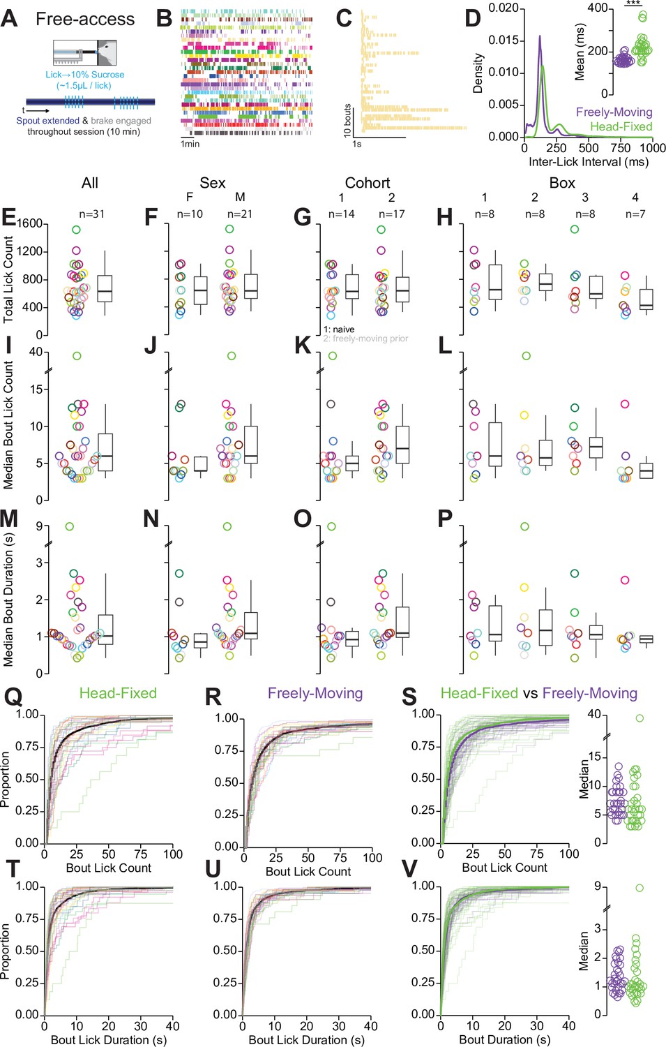
Quantification of behavior during head-fixed spout training.
(A) Cartoon depicting the task design for head-fixed, free-access consumption of sucrose (free-access lick training). (B) Raster of all licks recorded in a single 10 min session for the 31 mice in the experiment (color indicates the mouse identity and is consistent with other plots depicting color-coded single mouse data). (C) Raster of all licking bouts for a representative mouse. (D) Density plot of inter-lick intervals in the head-fixed (green) and freely moving (purple) versions of free-access consumption. Inset shows the median inter-lick interval for all 31 mice in both versions of the task [paired Student’s t-test, t(30)=6.22, p=7.62e-7***]. (E–P) Summaries of licking behavior during free access in the head-fixed version of the task depicting the total lick count (E–H), median lick count per licking bout (I–L), and median duration per licking bout (M–P). Each row contains the same data from 31 mice divided by sex, cohort (1: naïve, 2: freely moving prior), and behavioral box number. No statistically significant differences in head-fixed free-access licking behavior were observed (sex and cohort effects assessed using a Welch two-sample unpaired t-test, box effect assessed using one-way ANOVA, see Source data 1 for a complete presentation of the statistical results). (Q–S) Cumulative distribution of the number of licks per bout in the head-fixed (Q) and freely moving (R) versions of the task. (S) Data from (Q) and (R) overlayed and color coded based on the version of the task (left) and the median values for each mouse in both versions of the task (right) indicating no differences in the median bout lick count (Welch two-sample t-test [paired, two-sided], t(30)=0.09, p=0.93). (T–V) Same as (Q–S) but for the duration of licking bouts (V right: Welch two-sample t-test [paired, two-sided], t(30)=-0.33, p=0.074). (Rings and faded lines depict individual mice.)
Figure 2—figure supplement 2
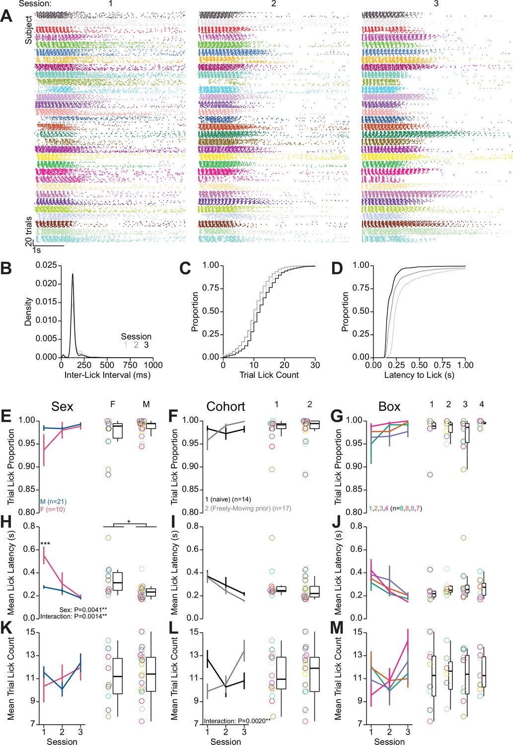
Quantification of behavior during head-fixed retractable spout training.
Further quantification of behavior during retractable spout training corresponding to data shown in Figure 2G–J. (A) Lick raster of all licks recorded across all trials across three sessions for the 31 mice in the experiment (color indicates the mouse identity and is consistent with other plots depicting color-coded single mouse data). (B) Density of inter-lick intervals. (C) Cumulative distributions of number of licks per trial. (D) Cumulative distribution of latency from spout extension command to first lick on trials with at least one lick. (E–M) Summaries of behavior during retractable spout training in each session (left) and averaged across sessions (right) depicting the proportion of trials with a lick (D–G), mean latency from spout extension to first lick (H–J), and mean number of licks per trial (K–M). Each row contains the same data from 31 mice divided by sex, cohort, and behavioral box (sex, cohort, and box effects over sessions were assessed using a using one-way repeated measures [RM] ANOVA, sex and cohort effects averaged across sessions assessed using Welch two-sample t-test [unpaired, two-sided], box effect averaged across sessions assessed using one-way ANOVA, statistically significant results are displayed on the relevant plots, asterisks above means indicate significant differences determined with honest significant difference (HSD) across group within the same session, see Source data 1 for a complete presentation of the statistical results). (Rings depict individual mice.)
Figure 2—figure supplement 3
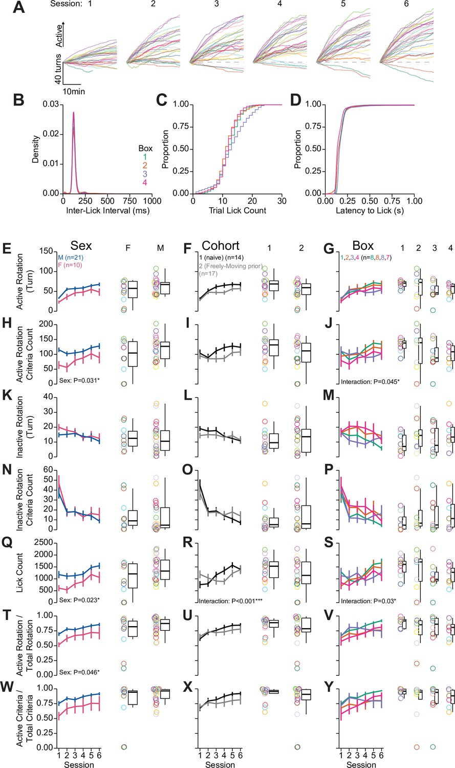
Quantification of behavior during head-fixed operant conditioning for sucrose.
Further quantification of behavior during operant training corresponding to data shown in Figure 2L–N. (A) Cumulative position of the wheel for all mice across all sessions. (B) Density of inter-lick intervals. (C) Cumulative distributions of number of licks per trial. (D) Cumulative distributions of latency from spout extension to first lick. (E–Y) Summaries of behavior during operant training depicting numerous metrics across each row. Each row contains the same data from 31 mice divided by sex, cohort, and behavioral box number. Line graphs depict mean and SEM for each session of training, the box and whisker plots with individual mice plotted as rings depict the mean over the last three sessions (sex, cohort, and box effects over sessions were assessed using a using one-way repeated measures [RM] ANOVA, sex and cohort effects averaged across sessions assessed using Welch two-sample t-test [unpaired, two-sided], box effect averaged across sessions assessed using one-way ANOVA, statistically significant results are displayed on the relevant plots, see Source data 1 for a complete presentation of the statistical results).
Figure 2—figure supplement 4

Comparison of head-fixed and freely moving versions of operant conditioning.
(A) The total rotation of the wheel across all sessions of operant conditioning in the head-fixed version of the task (numbers on the top of the plot indicate the fixed-ratio cost of reward in wheel turns; data in the last three sessions of 0.5 and 1.0 correspond to data presented in Figure 2N). (B) The nose poke count across all sessions of operant conditioning in the freely moving version of the task (numbers on top of the plot indicate the fixed-ratio cost of reward in nose pokes). (C) Mean z-score across the last three sessions of responding during the low (0.5 turn/3 nose pokes) and high (1.0 turn/5 nose pokes) cost sessions (three-way repeated measures [RM] ANOVA, system effect, F(1,30)=0.16, p=0.69, cost effect, F(1,30)=105.26, ***p=2.51e-11, response ID effect, F(1,30)=46.58, ***p=1.43e-7, system × cost interaction, F(1,30)=0.14, p=0.71, system × response ID interaction, F(1,30)=0.03, p=0.86, cost × response ID interaction, F(1,30)=47.24, ***p=1.25e-7, system × cost × response ID interaction, F(1,30)=13.86, ***p=8.13e-4, honest significant difference (HSD) post hoc, ***p<0.01, comparisons within a response and system; no significant difference between systems at any cost with the same particular response [e.g. head-fixed active low vs freely moving active low]). (D) Mean z-score of the active response during 5 min bins within the last three sessions of high-cost sessions (two-way RM ANOVA, system effect, F(1,30)=0.0, p=1.0, time effect, F(5,150)=430.01, p=5.41e-87, system × time interaction, F(5,150)=16.5, p=5.85e-13, HSD post hoc, ***p<0.001, *p<0.05, for comparisons across systems at the same time bin). (E) Average total body weight gain (liquid consumption) during the head-fixed and freely moving sessions indicating greater weight gain during the freely moving version of the task (Welch two-sample t-test [paired, two-sided], t(30)=4.38, p=1.35e-4). (Color in A and B indicates the response id, color in C and D indicates system, see Source data 1 for a complete presentation of the statistical results.)
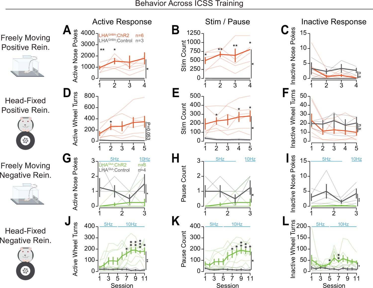
Figure 3 with 4 supplements
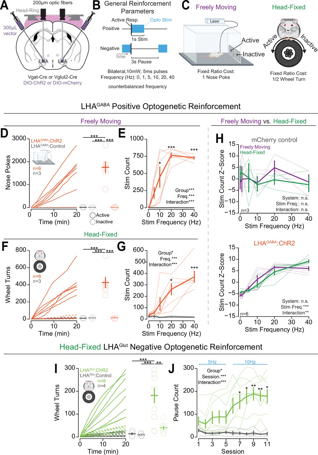
Head-fixed operant conditioning to obtain stimulation of lateral hypothalamic area GABAergic (LHAGABA) neurons or avoid stimulation of LHA glutamatergic (LHAGlut) neurons.
(A) Approach, placements depicted in Figure 3—figure supplement 1A. (B) Diagram of the experimental approach for positive reinforcement conducted with LHAGABA mice and negative reinforcement conducted with LHAGlut mice. (C) Cartoon depicting the freely moving (left) and head-fixed (right) versions of the operant task. (D) Cumulative (left) and total (right) freely moving nose pokes under positive reinforcement for 40 Hz stimulation in LHAGABA:ChR2 (red) and LHAGABA:Control (gray) mice (two-way repeated measures [RM] ANOVA, group effect, F(1,7)=22.15, **p=0.0022, response ID effect, F(1,7)=22.21, **p=0.0022, group × response ID interaction, F(1,7)=22.19, **p=0.0022, honest significant difference (HSD) post hoc, ***p<0.001). (E) Total number of stimulations earned under positive reinforcement within the freely moving task for different stimulation frequencies (two-way RM ANOVA, group effect, F(1,7)=31.89, ***p=7.7e-4, frequency effect, F(5,35)=12.25, ***p=6.7E-7, group × frequency interaction, F(5,35)=12.33, ***p=6.8e-7, HSD post hoc, *p<0.05, ***p<0.001). (F) Cumulative (left) and total (right) head-fixed wheel turns under positive reinforcement for 40 Hz stimulation in LHAGABA:ChR2 (red) and LHAGABA:Control (gray) mice (two-way RM ANOVA, group effect, F(1,7)=15.98, **p=0.0052, response ID effect, F(1,7)=22.01, **p=0.0022, group × response ID interaction, F(1,7)=22.78, **p=0.0020, HSD post hoc, ***p<0.001). (G) Total number of stimulations earned under positive reinforcement within the head-fixed task for different stimulation frequencies (two-way RM ANOVA, group effect, F(1,7)=11.00, *p=0.013, frequency effect, F(5,35)=9.00, ***p=1.44e-5, group × frequency interaction, F(5,35)=9.50, ***p=8.6e-6, HSD post hoc, *p<0.05, ***p<0.001). (H) Comparisons of the z-score of the total number of stimulations across frequencies in freely moving (purple) and head-fixed (green) in LHAGABA:Control mice (top, two-way RM ANOVA, system effect, F(1,2)=0.00, p=1.00, frequency effect, F(5,10)=0.27, p=0.92, system × frequency interaction, F(5,10)=0.68, p=0.65, HSD post hoc) and LHAGABA:ChR2 mice (bottom, two-way RM ANOVA, system effect, F(1,5)=0.00, p=1.00, frequency effect, F(5,25)=42.68, ***p=1.88e-11, system × frequency interaction, F(5,25)=4.37, p=5.38e-3, HSD post hoc, no significant post hoc differences when comparing systems at the same stimulation frequency). (I) Cumulative rotation over a session under negative reinforcement for 5 Hz and 10 Hz stimulation in LHAGlut:ChR2 (lime green) and LHAGlut:Control (gray) mice (two-way RM ANOVA, group effect, F(1,10)=13.78, **p=0.0040, response id effect, F(1,10)=9.07, *p=0.013, group × response ID interaction, F(1,10)=8.03, *p=0.018, HSD post hoc, **p<0.01, ***p<0.001). (J) Total pause count across all training sessions during negative reinforcement at the frequency indicated with blue text above the plot (two-way RM ANOVA, group effect, F(1,10)=8.71, *p=0.015, session effect, F(10,100)=5.67, ***p=1.18E-6, group × session interaction, F(10,100)=6.88, ***p=4.22E-8, Bonferroni adjusted t-test post hoc, *p<0.05, **p<0.01). (Faded lines and rings depict individual mice; asterisks above means indicate significant differences determined between stim count at a corresponding stim frequency or pause count at a corresponding session; asterisks above horizontal lines indicate significant difference determined between means indicated by edges of corresponding line; see Source data 1 for a complete presentation of the statistical results.)
Figure 3—figure supplement 1
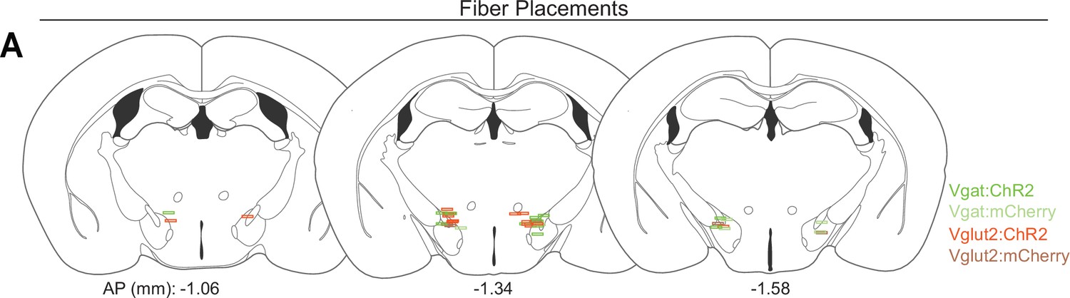
Placement of optic fibers.
(A) Histological locations relative to bregma of the tip of optic fibers targeting the lateral hypothalamic area (LHA). Colors indicate the experimental group of the corresponding mouse.
Figure 3—figure supplement 2
Training data for operant conditioning to obtain or avoid optogenetic stimulation.
Training data across training for each stage of the task with counts for active responses (left column), stimulations or pauses (mid column), and inactive responses (right column). (A–C) Behavior across training in positive reinforcement for optogenetic stimulation of LHAGABA neurons using the freely moving system. (A) Active nose pokes across training (two-way repeated measures [RM] ANOVA, group effect, F(1,7)=7.44, *p=0.029, session effect F(3,21)=0.74, p=0.54, group × session interaction, F(3,21)=0.75, p=0.54). (B) Stimulation count across training (two-way RM ANOVA, group effect, F(1,7)=14.67, **p=0.0065, session effect F(3,21)=1.28, p=0.31, group × session interaction, F(3,21)=1.3, p=0.30). (C) Inactive nose pokes across training (two-way RM ANOVA, group effect, F(1,7)=2.99, p=0.13, session effect F(3,21)=1.29, p=0.30, group × session interaction, F(3,21)=0.56, p=0.65). (D–F) Behavior across training in positive reinforcement for optogenetic stimulation of LHAGABA neurons using OHRBETS (Open-Source Head-fixed Rodent Behavioral Experimental Training System). (D) Active rotation across training (two-way RM ANOVA, group effect, F(1,7)=5.4, p=0.053, session effect, F(4,28)=2.32, p=0.082, group × session interaction, F(4,28)=2.73, *p=0.049). (E) Stimulation count across training (two-way RM ANOVA, group effect, F(1,7)=8.36, *p=0.023, session effect, F(4,28)=0.57, p=0.69, group × session interaction, F(4,28)=1.2, p=0.33). (F) Inactive rotation across training (two-way RM ANOVA, group effect, F(1,7)=0.74, p=0.42, session effect, F(4,28)=1.35, p=0.27, group × session interaction, F(4,28)=1.37, p=0.27). (G–I) Behavior across training in negative reinforcement for optogenetic stimulation of LHAGlut neurons using the freely moving system. (G) Active nose pokes across training (two-way RM ANOVA, group effect, F(1,10)=9.07, *p=0.013, session effect, F(3,30)=1.52, p=0.23, group × session interaction, F(3,30)=1.99, p=0.14). (H) Pause count across training (two-way RM ANOVA, group effect, F(1,10)=9.78, *p=0.011, session effect, F(3,30)=1.12, p=0.36, group × session interaction, F(3,30)=1.48, p=0.24). (I) Inactive nose pokes across training (two-way RM ANOVA, group effect, F(1,10)=14.61, **p=0.0034, session effect, F(3,30)=3.58, *p=0.025, group × session interaction, F(3,30)=4.22, *p=0.013). (J–L) Behavior across training in negative reinforcement for optogenetic stimulation of LHAGlut neurons using OHRBETS. (J) Active rotation across training (two-way RM ANOVA, group effect, F(1,10)=11.8, **p=0.0064, session effect, F(10,100)=3.34, ***p=6.76e-4, group × session interaction, F(10,100)=4.21, ***p=6.98e-5). (K) Pause count across training (two-way RM ANOVA, group effect, F(1,10)=8.71, *p=0.015, session effect, F(10,100)=5.64, ***p=1.18e-6, group × session interaction, F(10,100)=6.88, ***p=4.22e-8). (L) Inactive rotation across training (two-way RM ANOVA, group effect, F(1,10)=6.06, *p=0.034, session effect, F(10,100)=0.81, p=0.62, group × session interaction, F(10,100)=1.02, p=0.43). (Faded lines depict individual mice; asterisks above means represent Bonferroni adjusted t-test comparisons between a group at a corresponding session [*p<0.05, **p<0.01, ***p<0.001]; see Source data 1 for a complete presentation of the statistical results.)
Figure 3—figure supplement 3
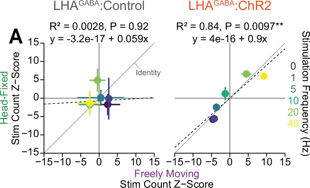
Correlation between freely moving and head-fixed stimulation count during positive reinforcement for lateral hypothalamic area GABAergic (LHAGABA) optogenetic stimulation.
(A) Correlation between the group mean z-score of stimulation counts during freely moving (abscissa) and head-fixed (ordinate) during positive reinforcement for optogenetic stimulation (error bars depict the standard error of the mean along each axis) (Pearson’s product-moment correlation, LHAGABA:Control, r=0.053, p=0.92, LHAGABA:ChR2, r=0.92, **p=9.72e-3).
Figure 3—figure supplement 4

Optogenetic stimulation gates responding under positive and negative reinforcement.
(A) Cumulative position over a 30 min session with the laser turned off from 10 to 20 min.
Figure 4 with 3 supplements
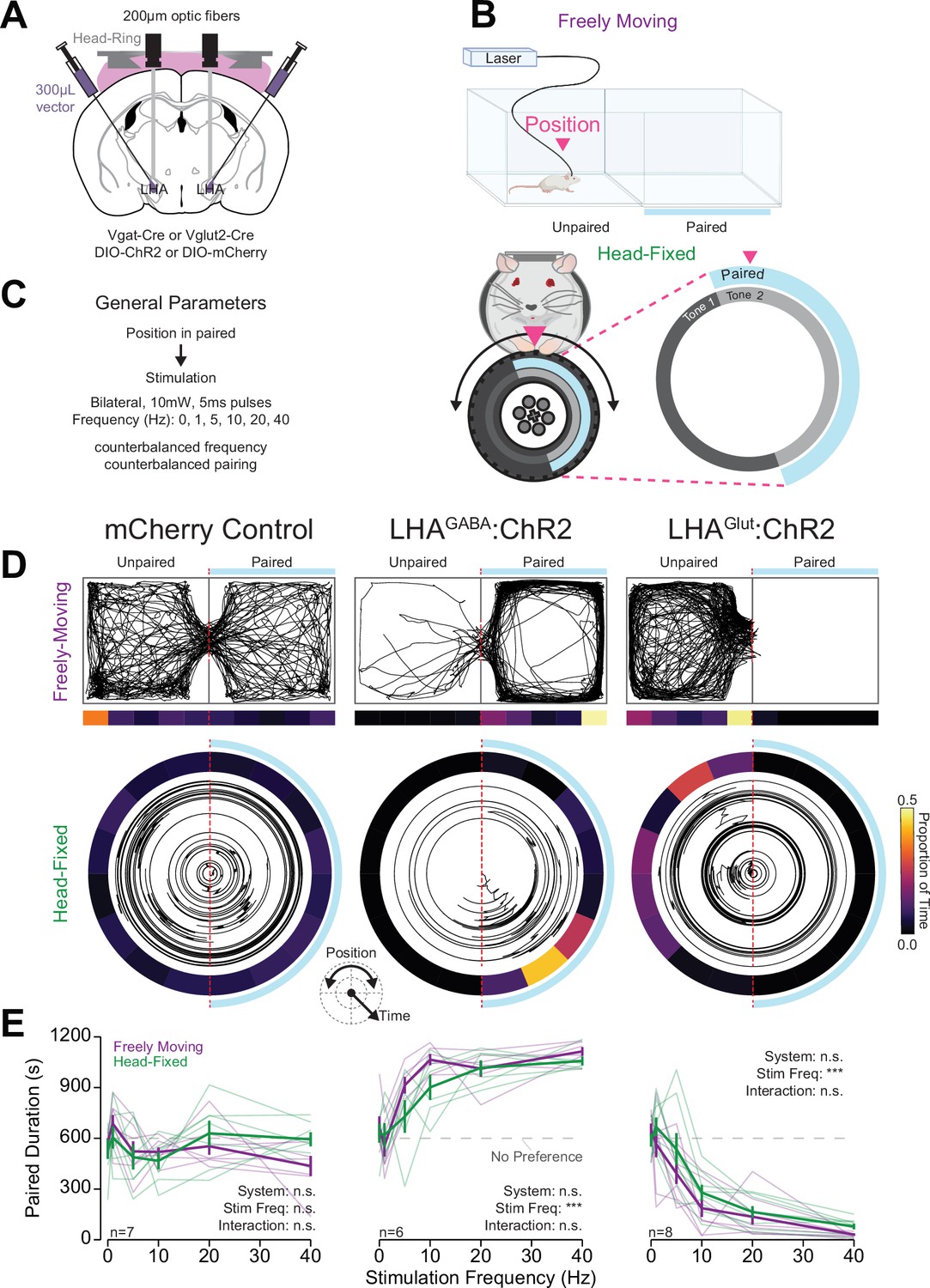
Head-fixed wheel time preference (WTP) and aversion associated with stimulation of lateral hypothalamic area (LHA) subpopulations mirrors freely moving behavior.
(A) Approach, placements depicted in Figure 3—figure supplement 1A. (B) Cartoon depicting the freely moving and head-fixed versions of the operant task. In the head-fixed task, the mouse’s position was determined relative to the position of the wheel and the mouse could rotate the wheel to navigate through the paired and unpaired zones. (C) Task design. (D–F) Behavior during the real-time place testing (RTPT) task; left column contains data from mCherry controls (both LHAGABA:Control and LHAGlut:Control), middle contains LHAGABA:ChR2, right contains LHAGlut:ChR2. (D) Representative traces of the mouse’s position in the two-chamber arena in freely moving RTPT (top) and the position of the wheel over time in head-fixed RTPT (bottom). The right side of the arena or wheel was paired with optogenetic stimulation as indicated by the blue bar/arc. The proportion of time in binned areas of the arena or wheel are shown in the heat maps under or surrounding the traces (color scale represents the proportion of time in each position bin). (E) Amount of time spent in the paired zone during a 20 min (1200 s) session for varying frequencies; values above 600 s are indicative of preference, values below are indicative of avoidance. Colors represent the behavioral system as indicated in the left column (two-way repeated measures [RM] ANOVA, mCherry control: system effect, F(1,6)=0.02, p=0.89, frequency effect, F(5,30)=2.25, p=0.075, system × frequency interaction, F(5,30)=1.42, p=0.25; LHAGABA:ChR2: system effect, F(1,5)=3.35, p=0.13, frequency effect, F(5,25)=19.49, ***p=6.65e-8, system × frequency interaction, F(5,25)=1.75, p=0.16; LHAGlut:ChR2: system effect, F(1,7)=4.01, p=0.085, frequency effect, F(5,35)=66.75, ***p=6.73e-17, system × frequency interaction, F(5,35)=1.18, p=0.34; no honest significant difference (HSD) differences between systems were detected at corresponding stimulation frequencies; see Source data 1 for a complete presentation of the statistical results).
Figure 4—figure supplement 1
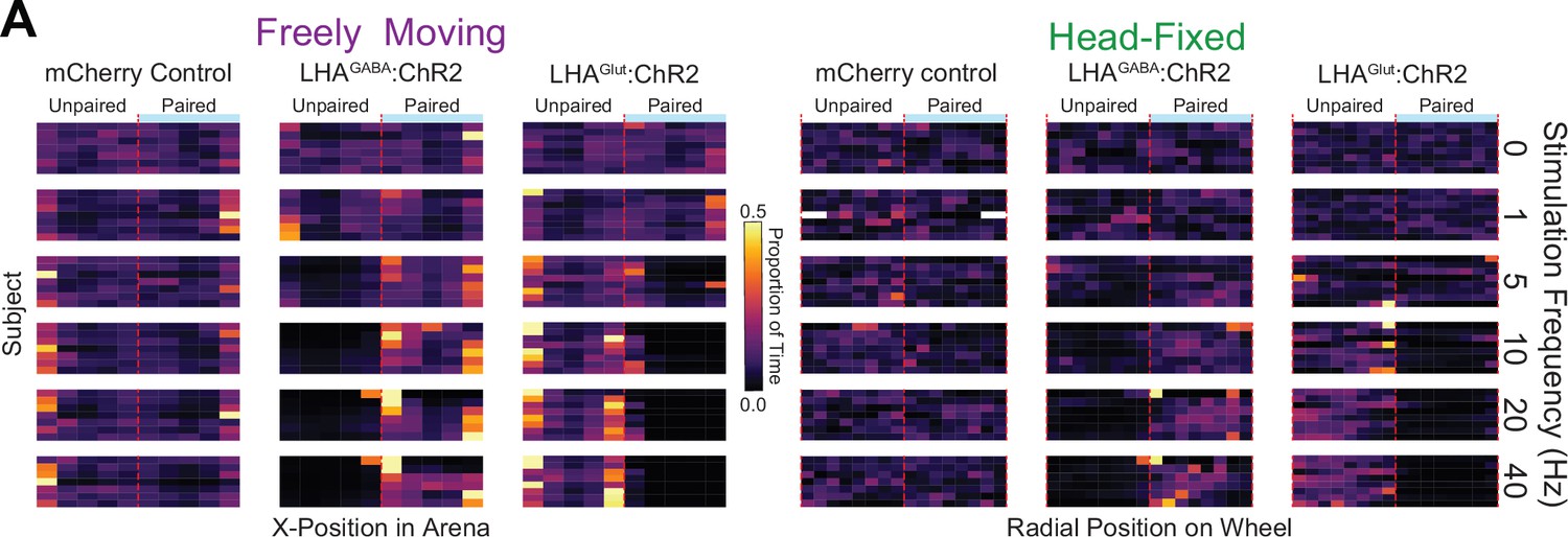
Single subject data in the wheel time preference (WTP) and real-time place testing (RTPT) assays.
(A) Heat map showing the binned x-position in the freely moving version of the task (left three columns) or radial position in the head-fixed version of the task (right three columns) of all mice across all stimulation frequencies (indicated by label on right). Color represents the proportion of time spent in the binned position. The paired side was counterbalanced across mice and sessions and is set to the right side for display purposes only.
Figure 4—figure supplement 2
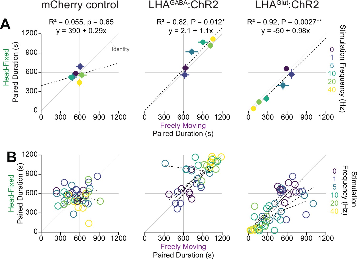
Correlation of behavior measured with the wheel time preference (WTP) and real-time place testing (RTPT) assays.
Correlation between the time spent in the paired zone during the freely moving (abscissa) or the head fixed (ordinate) at different stimulation frequencies represented as different colors for the group mean (A, Pearson’s product-moment correlation, mCherry control, r=0.23, p=0.65, LHAGABA:ChR2, r=0.91, *p=0.012, LHAGlut:ChR2, r=0.96, **p=0.27e-3) and individual subject (B, see the Source data 1 for a complete presentation of the statistical results).
Figure 4—figure supplement 3
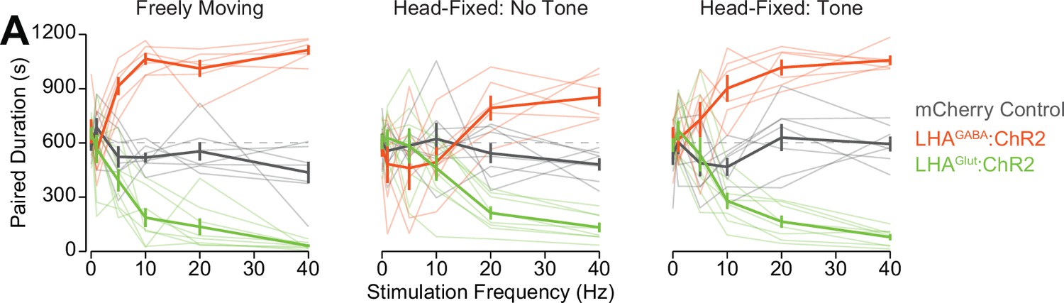
Behavior in the wheel time preference (WTP) with and without an auditory tone.
(A) Amount of time spent in the paired zone across the freely moving (left), head fixed without a tone indicating the area the mouse was located in (middle), and head-fixed with a tone indicating the area the mouse was located in (right).
Figure 5 with 4 supplements
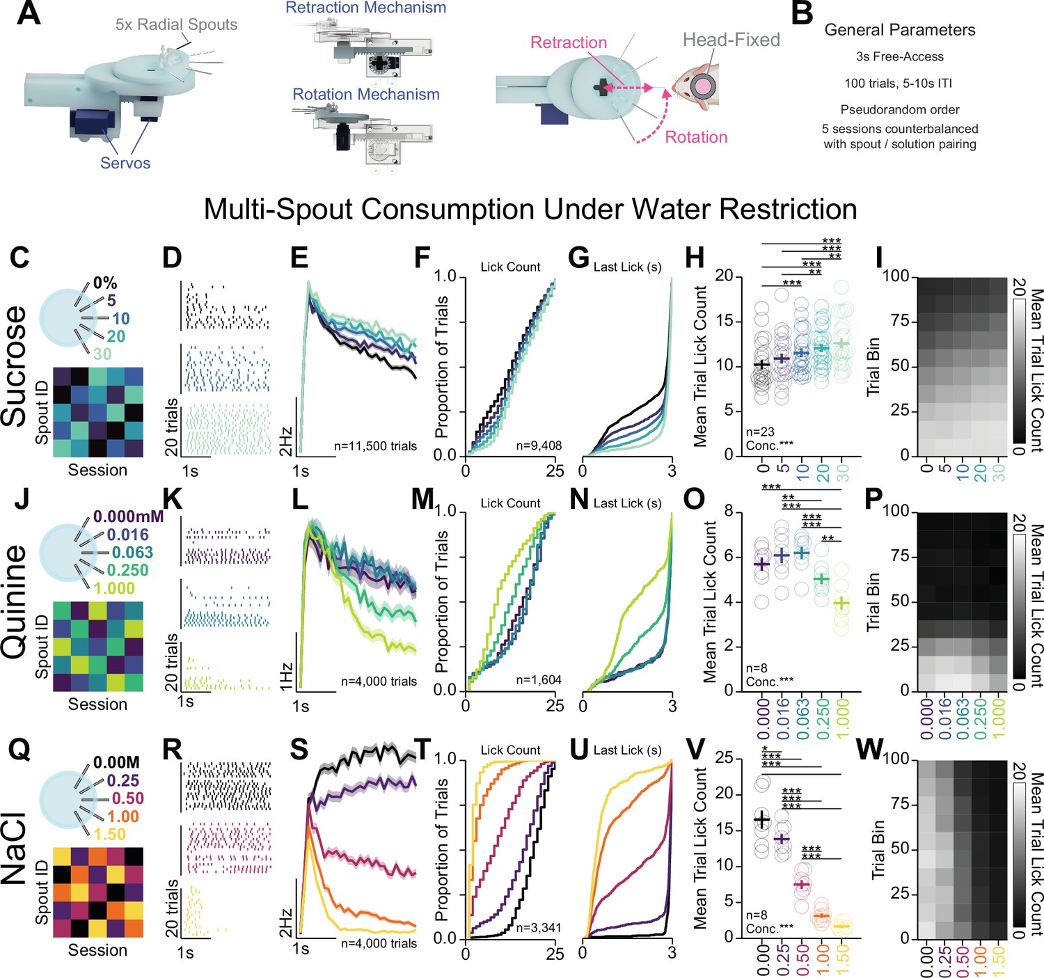
Head-fixed consumption of gradients of rewarding and aversive solutions during brief access.
(A) 3D rendering of the multi-spout unit that retracts and rotates to allow brief-access periods to one of five lick spouts to the head-fixed mouse. (B) Task design. (C–I) Multi-spout consumption of a gradient of concentrations of sucrose data. (C) Procedure: mice received five sessions of 5× multi-spout counterbalanced to have each solution of each spout once. Colors represent concentrations of solution as defined in the label adjacent to the multi-spout cartoon. (D) Lick raster of a representative mouse depicting the licks for water, medium concentration, and high concentration during the 3 s access period. (E) Mean binned lick rate for all mice for each concentration. (F–G) Cumulative distribution of the number of licks in trials with a lick (F) and the time of the last lick within each licking bout (G). (H) The mean number of licks per trial for each concentration (one-way repeated measures [RM] ANOVA, concentration effect, F(4,88)=19.18, ***p=2.26e-11, honest significant difference (HSD) post hoc, ***p<0.001, **p<0.01). (I) The mean number of licks for each concentration per trial binned by 10 trials over the course of the session. (J–P) same as (C–I), but for data from multi-spout consumption of a gradient of concentrations of quinine (one-way RM ANOVA, concentration effect, F(4,28)=27.36, ***p=2.58E-9, HSD post hoc, ***p<0.001, **p<0.01). (Q–W) same as (C–I), but for data from multi-spout consumption of a gradient of concentrations of NaCl (one-way RM ANOVA, concentration effect, F(4,28)=140.16, ***p=4.35e-18, HSD post hoc, ***p<0.001, **p<0.01, *p<0.05). (Asterisks depict post hoc comparisons between concentrations indicated by edges of corresponding horizontal line; faded lines depict individual mice; see Source data 1 for a complete presentation of the statistical results.)
Figure 5—figure supplement 1
Quantification of head-fixed consumption during brief access.
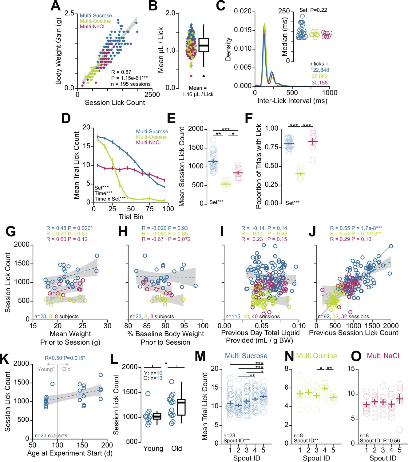
(A) Correlation between the number of licks and body weight gain within each session (Pearson’s product-moment correlation, r=0.87, ***p=1.15e-61). (B) Estimated volume consumed per lick produced by dividing the body weight gain by the number of licks within the session. (C) Density plot of inter-lick intervals within each session set. Inset shows the median inter-lick interval (one-way ANOVA, solution set effect, F(2,36)=1.56, p=0.22). (D) Mean trial lick count across all concentrations in bins of 10 trials across the session for each solution set (two-way repeated measures [RM] ANOVA, solution set effect, F(2,36)=31.47, ***p=1.25e-8, trial bin effect, F(9,324)=187.87, ***p=7.01e-123, solution set × trial bin interaction, F(18,324)=34.86, ***p=8.67e-65). (E) Mean total number of licks for sessions for each solution set (one-way ANOVA, solution set effect, F(2,36)=31.47, ***p=1.25e-8, honest significant difference (HSD) post hoc, *p<0.05, **p<0.01, ***p<0.001). (F) Proportion of trials with at least one lick for each solution set (one-way ANOVA, solution set effect, F(2,36)=103.3, ***p=1.22e-15, HSD post hoc, ***p<0.001). (G–J) Correlations between different factors (abscissa) and session lick count (ordinate): (G) mean weight prior to the session (Pearson’s product-moment correlation, multi-sucrose r=0.48, *p=0.020, multi-quinine r=0.20, p=0.63, multi-NaCl r=0.60, p=0.12). (H) Percent baseline body weight prior to the session (Pearson’s product-moment correlation, multi-sucrose r=−0.020, p=0.93, multi-quinine r=−0.080, p=0.85, multi-NaCl r=−0.67, p=0.072). (I) Total liquid consumed+provided to the mouse on the session prior to the session (Pearson’s product-moment correlation, multi-sucrose r=−0.14, p=0.14, multi-quinine r=−0.11, p=0.48, multi-NaCl r=0.23, p=0.15). (J) The lick count on the previous session (Pearson’s product-moment correlation, multi-sucrose r=0.55, ***p=1.7e-8, multi-quinine r=0.54, **p=1.3e-3, multi-NaCl r=0.29, p=0.10). (K) Correlation between the age of the mouse at the experiment start (abscissa) and session lick count (ordinate) during the multi-spout consumption of a gradient of sucrose concentrations (Pearson’s product-moment correlation, r=0.50, *p=0.015, mice used in multi-spout consumption of a gradient of NaCl concentrations and quinine concentrations did not have enough variance in age to conduct this analysis). (L) Mean session lick count in mice defined as young (<100 days at start of experiment) and old (>100 days at start of experiment) (Welch two-sample t-test [unpaired, two-sided], t(21)=2.19, *p=0.015). (M–O) Mean trial lick count across spouts for data presented in Figure 5. (M) Multi-sucrose (one-way RM ANOVA, spout effect, F(4,88)=9.62, ***p=1.68e-6, HSD post hoc, *p<0.05, **p<0.01, ***p<0.001). (N) Multi-quinine (one-way RM ANOVA, spout effect, F(4,28)=4.83, **p=4.34e-3, HSD post hoc, *p<0.05, **p<0.01). (O) Multi-NaCl (one-way RM ANOVA, spout effect, F(4,28)=0.77, p=0.56). (Asterisks depict HSD comparisons indicated by horizontal lines; faded lines and rings depict individual mice; see Source data 1 for a complete presentation of the statistical results.)
Figure 5—figure supplement 2

Multi-spout consumption of different gradients of concentrations of quinine.
Analysis of three gradients of concentrations of quinine. Each concentration set had water and four concentrations of quinine with a 1:4 serial dilution starting at 1 mM (low), 5 mM (med), and 10 mM (high). (A–C) Left, middle, and right columns depict data from low, med, and high concentration sets of quinine. (A) Mean binned lick rate for all mice for each concentration. (B) The mean number of licks per trial for each concentration (one-way repeated measures [RM] ANOVA, concentration effect, low (1 mM), F(4,28)=27.36, ***p=2.58e-9, med (5 mM), F(4,28)=33.78, ***p=2.43e-10, high (10 mM), F(4,28)=16.37, ***p=5.06e-7, honest significant difference (HSD) post hoc, *p<0.05, **p<0.01, ***p<0.001). (C) The mean number of licks for each concentration per trial binned by 10 trials over the course of the session. (D) The mean number of licks per trial for quinine concentrations greater than 0 shown on a log scale of quinine concentration on the abscissa. (E) Mean session lick count for each concentration set (one-way RM ANOVA, quinine set effect, F(2,14)=8.71, **p=3.49e-3, HSD post hoc, **p<0.01). (F) Proportion of trials with a lick for each concentration set (one-way RM ANOVA, quinine set effect, F(2,14)=2.96, p=0.084). (Asterisks depict HSD comparisons indicated by horizontal lines; faded rings depict individual mice; see Source data 1 for a complete presentation of the statistical results.)
Figure 5—figure supplement 3

Sex differences in head-fixed multi-spout consumption behavior.
Investigation of potential sex effects on behavior in the multi-spout brief-access assay shown in Figure 5. (A–B) Consumption of a gradient of concentrations of sucrose. (A) The mean number of licks per trial for each concentration (two-way repeated measures [RM] ANOVA, sex effect, F(1,21)=0.97, p=0.34, concentration effect, F(4,84)=20.38, ***p=9.24e-12, sex × concentration interaction, F(4,84)=1.57, p=0.19). (B) Mean total lick count per session (Welch two-sample t-test [unpaired, two-sided], t(19)=0.97, p=0.34). (C) Proportion of trials with a lick (Welch two-sample t-test [unpaired, two-sided], t(21)=2.21, *p=0.039). (D–F) same as (A–B), but for consumption of a gradient of concentrations of quinine. (D) (two-way RM ANOVA, sex effect, F(1,6)=0.02, p=0.90, concentration effect, F(4,24)=27.09, ***p=1.37e-8, sex × concentration interaction, F(4,24)=0.93, p=0.46). (E) Mean total lick count per session (Welch two-sample t-test [unpaired, two-sided], t(4)=0.13, p=0.90). (F) Proportion of trials with a lick (Welch two-sample t-test [unpaired, two-sided], t(5)=0.60, p=0.58). (G–I) same as (A–B), but for consumption of a gradient of concentrations of NaCl. (G) Two-way RM ANOVA, sex effect, F(1,6)=2.92, p=0.14, concentration effect, F(4,24)=124.85, ***p=1.1e-15, sex × concentration interaction, F(4,24)=0.24, p=0.92. (H) Mean total lick count per session (Welch two-sample t-test [unpaired, two-sided], t(6)=1.71, p=0.14). (I) Proportion of trials with a lick (Welch two-sample t-test [unpaired, two-sided], t(4)=3.06, *p=0.039). (See Source data 1 for a complete presentation of the statistical results.)
Figure 5—figure supplement 4

Potential anticipation of solution identity.
Proportion of trials with a lick response in mice under water restriction during multi-spout brief-access consumption. Mice do not show of anticipation for sucrose (A, one-way RM ANOVA, concentration effect, F(4,88)=0.99, p=0.42), or quinine (B, one-way RM ANOVA, concentration effect, F(4,28)=0.59, p=0.67), but show anticipation of NaCl (C, one-way RM ANOVA, concentration effect, F(4,28)=11.39, ***p=1.29e-5, honest significant difference (HSD) post hoc, ***p<0.001). (See Source data 1 for a complete presentation of the statistical results.)
Figure 6 with 1 supplement
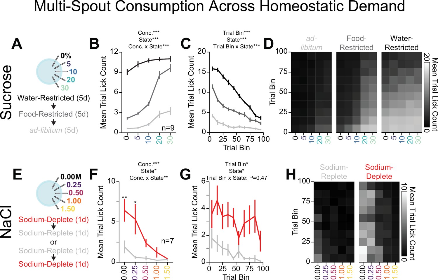
Homeostatic demand shifts within session consumption of gradients of sucrose and NaCl.
(A) Procedure: Mice ran sequentially through water restriction, food restriction, and ad libitum states and during each state, mice received five sessions of multi-spout counterbalanced to have each concentration of sucrose on each spout once (two-way repeated measures [RM] ANOVA, concentration effect, F(4,32)=157.23, ***p=1.48e-20, demand state, F(2,16)=542.04, ***p=2e-15, concentration × demand state interaction, F(8,64)=33.84, ***p=3.59e-20, honest significant difference [HSD] post hoc, every mean is significantly different from every other, except 30% sucrose consumption under food and water restriction). (B) The mean number of licks per trial for each concentration of sucrose in the ad libitum (light gray), food-restricted (dark gray), and water-restricted (black) states (two-way RM ANOVA, trial bin, F(9,72)=149.63, ***p=6.19e-43, demand state, F(2,16)=542.04, ***p=2e-15, trial bin × demand state interaction, F(18,144)=35.43, ***p=7.32e-44). (C) Mean trial lick count across all concentrations of sucrose in bins of 10 trials across the session for each homeostatic state. (D) The mean number of licks for each concentration of sucrose per trial binned by 10 trials over the course of the session for each homeostatic state. (E) Procedure: In sodium-replete or sodium-deplete states in counterbalanced order, mice received one session of multi-spout with a gradient of concentrations of NaCl. The pairing of solution concentrations and spouts remained consistent. (F) The mean number of licks per trial for each concentration of NaCl in the sodium-replete (gray) and -deplete (red) states (two-way RM ANOVA, concentration effect, F(4,24)=9.04, ***p=1.33e-4, demand state, F(1,6)=13.19, *p=0.011, concentration × demand state interaction, F(4,24)=4.41, **p=8.2e-3, HSD post hoc, **p<0.01, *p<0.05). (G) Mean trial lick count across all concentrations of NaCl in bins of 10 trials across the session for each homeostatic state (two-way RM ANOVA, trial bin, F(9,54)=2.57, *p=0.016, demand state, F(1,6)=12.76, *p=0.012 trial bin × demand state interaction, F(9,54)=0.98, p=0.47). (H) The mean number of licks for each concentration of NaCl per trial binned by 10 trials over the course of the session for each homeostatic state. (Asterisks above means indicate differences between homeostatic demand state at a corresponding concentration; see Source data 1 for a complete presentation of the statistical results.)
Figure 6—figure supplement 1
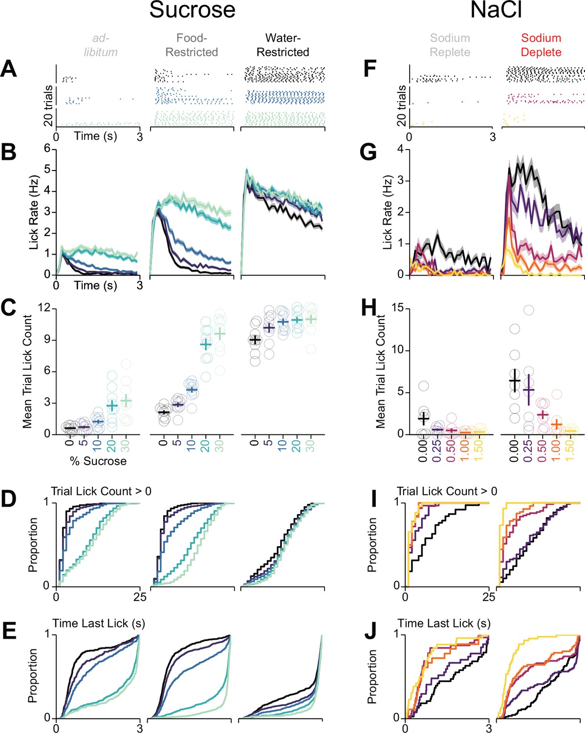
Behavioral details for differences in consumption across homeostatic demand.
Sets of columns containing data from mice in Figure 6 undergoing multi-spout consumption of a gradient of concentrations of sucrose (left three columns) or NaCl (right two columns) across homeostatic demands. (A) Lick raster of a representative mouse depicting the licks for water, medium concentration, and high concentration during the 3 s access period. (B) Mean binned lick rate for all mice for each concentration. (C) The mean number of licks per trial for each concentration (same data as Figure 6 but with single mice displayed). (D–E) Cumulative distribution of the number of licks in trials with a lick (D) and the time of the last lick within each licking bout (E). (F–J) same as (A–E), but for consumption of a gradient of concentrations of NaCl.
Figure 7 with 1 supplement
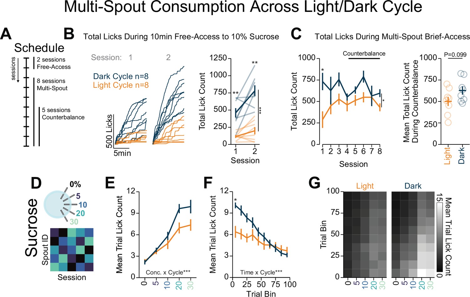
Light/dark cycle shifts within-session consumption of gradients of sucrose.
(A) Schedule for behavioral sessions. (B) Licking behavior during two sessions of free-access licking for 10% sucrose displayed as cumulative licking (left) and total lick count during the session (right). During free-access training, mice tested in the dark cycle licked more than mice tested in the light cycle (two-way repeated measures [RM] ANOVA, cycle effect, F(1,14)=58.52, ***p=2.30e-6, session effect, F(1,14)=11.93, **p=3.87e-3, cycle × session interaction, F(1,14)=4.13, p=6.15e-2, honest significant difference (HSD) post hoc, **p<0.01). (C) Total licking behavior during eight sessions of multi-spout brief access to a gradient of sucrose concentration (left) and mean over five counterbalance sessions (right). Mice tested in the dark cycle licked more than mice tested in the light cycle over all eight sessions (two-way RM ANOVA, cycle effect, F(1,14)=5.24, *p=0.38, session effect, F(7,98)=1.84, p=0.088, cycle × session interaction, F(7,98)=1.97, p=0.066, HSD post hoc, *p<0.05), but not over the five counterbalanced sessions (sessions 4–8, Welch two-sample t-test [paired, two-sided], t(14)=3.17, p=0.099). (D) Procedure: Mice were trained in five sessions of sucrose multi-spout counterbalanced to have each solution paired with each spout once. (E) Mean number of licks per trial for each concentration of sucrose for mice ran in the dark cycle (blue) and mice ran in the light cycle (orange) (two-way RM ANOVA, cycle effect, F(1,14)=3.17, p=0.097, concentration effect, F(4,56)=104, ***p=3.08e-25, cycle × concentration interaction, F(4,56)=5.72, ***p=6.26e-4). (F) Mean trial lick count across all concentrations of sucrose in bins of 10 trials across the session (two-way RM ANOVA, cycle effect, F(1,14)=3.15, p=0.097, time effect, F(9,96)=42.6, ***p=4.36e-34, cycle × time interaction, F(9,96)=9.19, ***p=1.3e-10, HSD post hoc *p<0.05). (G) The mean number of licks for each concentration of sucrose per trial binned by 10 trials over the course of the session. (Asterisks above means indicate differences between mice tested in each cycle during the same session.)
Figure 7—figure supplement 1

Comparison of multi-spout behavior across labs.
(A) Data included in figure: Comparison between mice that were food-restricted and ran through multi-spout brief access to a gradient of sucrose concentrations in the dark cycle in the Stuber lab (data shown in Figure 6) and the Roitman lab (data shown in Figure 7). (B) Mean binned lick rate for all mice for each concentration indicated by color with facets for lab (left) and for each lab indicated by color with facets for sucrose concentration (right). (C) Density plot of inter-lick intervals for mice ran in the Stuber and Roitman labs indicating a higher density of low inter-lick intervals in mice ran in the Roitman lab compared to the Stuber lab. Inset shows the median inter-lick interval (Welch two-sample t-test [unpaired, two-sided], t(9)=3.29, **p=9.89e-3). (D) The mean number of licks per trial for each concentration of sucrose for mice ran in the Stuber and Roitman labs indicating no effect of lab (two-way RM ANOVA, lab effect, F(1,15)=1.87, p=0.19, concentration effect, F(4,60)=229.45, ***p=1.26e-35, lab × concentration interaction, F(4,60)=1.88, p=0.13, see Source data 1 for a complete presentation of the statistical results).
Figure 8 with 6 supplements
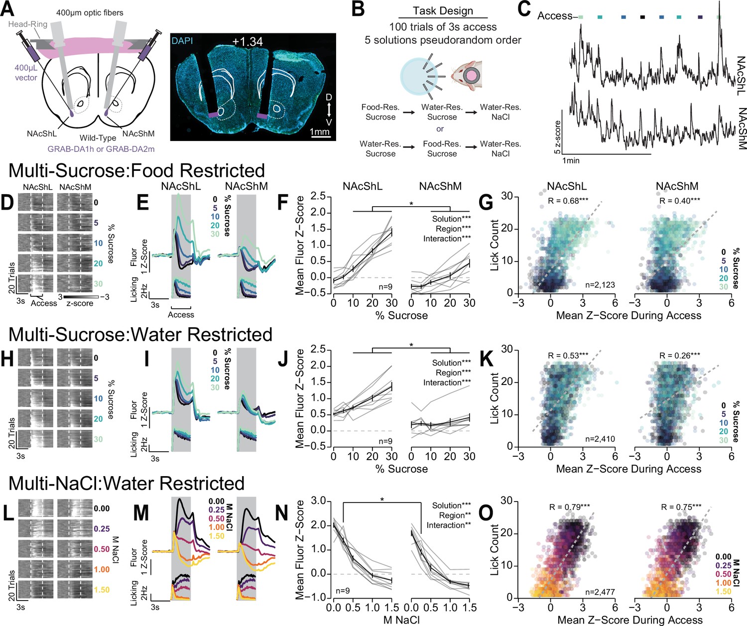
Differential dopamine dynamics during multi-spout consumption behavior.
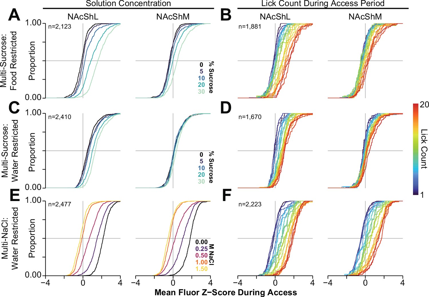
(A) Approach for simultaneously recording dopamine dynamics in the lateral nucleus accumbens shell (NAcShL) and medial nucleus accumbens shell (NAcShM) (left), and representative placements of optic fibers overlaying the NAcSh (white numerical value indicates AP position relative to bregma). (B) Task design and schedule of experiment. (C) Representative trace of simultaneous GRAB-DA fluorescence in the NAcShM and NAcShL during multi-spout access to sucrose under food restriction (lines on top indicate access periods, color indicates sucrose concentration). (D–G) Dopamine dynamics during multi-sucrose under food restriction: (D) Representative heat map of GRAB-DA fluorescence over time during each trial sorted by sucrose concentration (trials averaged over three sessions of recording, earliest trails depicted on bottom). (E) Perievent time histograms of mean GRAB-DA fluorescence (top) and licks (bottom) separated by sucrose concentration. (F) Mean fluorescence z-score during access period indicating strong scaling in the NAcShL (left) and weak scaling in the NAcShM (right) (two-way repeated measures [RM] ANOVA, concentration effect, F(4,32)=71.29, ***p=1.77e-15, brain region effect, F(1,8)=51.63, ***p=9.38e-5, concentration × brain region interaction, F(4,32)=14.94, ***p=5.46e-7, honest significant difference (HSD) post hoc, *p<0.05 NAcShL vs NAcShM at same concentration). (G) On individual trials, the mean z-score during access correlates with licking in both the NAcShL (left) and NAcShM (right) (color depicts the solution concentration) (Pearson’s product-moment correlation, NAcShL, r=0.68, ***p=2.06e-292, NacShM, r=0.40, ***p=5.08e-82). (H–K) Same as D–G for dopamine dynamics during multi-sucrose under water restriction. (H) Representative heat map of GRAB-DA fluorescence over time during each trial sorted by sucrose concentration (trials averaged over three sessions of recording, earliest trails depicted on bottom). (I) Perievent time histograms of mean GRAB-DA fluorescence (top) and licks (bottom) separated by sucrose concentration. (J) Mean fluorescence z-score during access period indicating moderate scaling in the NAcShL (left) and weak scaling in the NAcShM (right) (two-way RM ANOVA, concentration effect, F(4,32)=20.81, ***p=1.57e-8, brain region effect, F(1,8)=27.82, ***p=7.51e-4, concentration × brain region interaction, F(4,32)=11.61, ***p=6.16e-6, HSD post hoc, *p<0.05 NAcShL vs NAcShM at same concentration). (K) On individual trials, the mean z-score during access correlates with licking in both the NAcShL (left) and NAcShM (right) (color depicts the solution concentration) (Pearson’s product-moment correlation, NAcShL, r=0.53, ***p=4.53e-173, NacShM, r=0.26, ***p=1.45e-37). (L–O) Same as D–G for dopamine dynamics during multi-NaCl under water restriction. (L) Representative heat map of GRAB-DA fluorescence over time during each trial sorted by NaCl concentration (trials averaged over three sessions of recording, earliest trails depicted on bottom). (M) Perievent time histograms of mean GRAB-DA fluorescence (top) and licks (bottom) separated by NaCl concentration. (N) Mean fluorescence z-score during access period indicating strong scaling in the NAcShL (left) and strong scaling in the NAcShM (right) (two-way RM ANOVA, concentration effect, F(4,32)=123.48, ***p=5.66e-19, brain region effect, F(1,8)=11.28, **p=0.010, concentration × brain region interaction, F(4,32)=4.53, **p=0.0052, HSD post hoc, *p<0.05 NAcShL vs NAcShM at same concentration). (O) On individual trials, the mean z-score during access correlates with licking in both the NAcShL (left) and NAcShM (right) (color depicts the solution concentration) (Pearson’s product-moment correlation, NAcShL, r=0.79, ***p<2.23e-308, NacShM, r=0.75, ***p<2.23e-308).
Figure 8—figure supplement 1

Multi-spout licking behavior.
Multi-spout licking behavior corresponding to Figure 8. (A) Mean binned lick rate for all mice for each concentration during multi-spout consumption of sucrose under food restriction (color indicates concentration of sucrose). (B) The mean number of licks per trial for each concentration of sucrose under food restriction (one-way repeated measures [RM] ANOVA, concentration effect, F(4,32)=128.96, p=2.95e-19). (C) Mean binned lick rate for all mice for each concentration during multi-spout consumption of sucrose under water restriction (color indicates concentration of sucrose). (D) The mean number of licks per trial for each concentration of sucrose under water restriction (one-way RM ANOVA, concentration effect, F(4,32)=16.66, p=1.77e-7). (E) Mean binned lick rate for all mice for each concentration during multi-spout consumption of NaCl under water restriction (color indicates concentration of NaCl). (F) The mean number of licks per trial for each concentration of NaCl under water restriction (one-way RM ANOVA, concentration effect, F(4,32)=120.44, p=8.21e-19). (See Source data 1 for a complete presentation of the statistical results.)
Figure 8—figure supplement 2
Cumulative distribution functions of GRAB-DA responses in the NAcSh during multi-spout consumption behavior.
Cumulative distribution functions of mean GRAB-DA fluorescence during the access period for all trials with at least one lick during multi-spout sucrose under food restriction grouped and colored by the trial solution (left column; A, C, E) or lick count (right column; B, D, F). Rows contain GRAB-DA signals during multi-spout sucrose under food restriction (A, B), multi-spout sucrose under water restriction (C, D), and multi-spout NaCl under water restriction (E, F) (color indicates solution or lick count as indicated by corresponding inset).
Figure 8—figure supplement 3

Linear correlation of dopamine dynamics during multi-spout consumption.
Correlations between medial nucleus accumbens shell (NAcShM) and lateral nucleus accumbens shell (NAcShL) mean GRAB-DA fluorescence during the access period for all trials with at least one lick during multi-sucrose under food restriction (A, Pearson’s product-moment correlation, r=0.69, ***p=1.24e-301), multi-sucrose under water restriction (B, Pearson’s product-moment correlation, r=0.61, ***p=1.23e-249), and multi-NaCl under water restriction (C, Pearson’s product-moment correlation, r=0.87, ***p<2.23e-308).
Figure 8—figure supplement 4

Range of licking and NAcSh dopamine signals during multi-spout consumption behavior.
(A) Range of licking (absolute difference in licking during access to highest and lowest concentrations) across each stage of the task (WR: water-restricted, FR: food-restricted) (one-way repeated measures [RM] ANOVA, stage effect, F(2,16)=189.39, ***p=7.28e-12). (B) Range of GRAB-DA fluorescence signals (absolute difference in mean z-score during access to highest and lowest concentrations) across each stage of the task (two-way RM ANOVA, brain region effect, F(1,8)=14.96, **p=4.76e-3, stage effect, F(2,16)=82.12, p=3.86e-9, brain region × stage interaction, F(2,16)=18.87, p=6.73e-12). (Asterisks over means indicate differences between medial nucleus accumbens shell [NAcShM] and lateral nucleus accumbens shell [NAcShL] at a corresponding stage; all comparisons across stages within a brain region are significant; see Source data 1 for a complete presentation of the statistical results.)
Figure 8—figure supplement 5

Representative full-session traces.
(A) Full-session raw traces from mouse abb11 across three sessions of multi-NaCl under water-restricted conditions (WR:NaCl). Both the 465 nm channel (used for GRAB-DA2m imaging) and the 405 nm channel (imprecise isosbestic) show a high degree of stability over the course of the session. (B) Zoomed-in portion of trace shown in (A). Note that the 405 nm channel shows negative deflections during positive deflections in the 465 nm channel, which is likely due to the fact that 405 nm differs from the isosbestic wavelength for GRAB-DA2m of 440 nm (Sun et al., 2020).
Figure 8—figure supplement 6
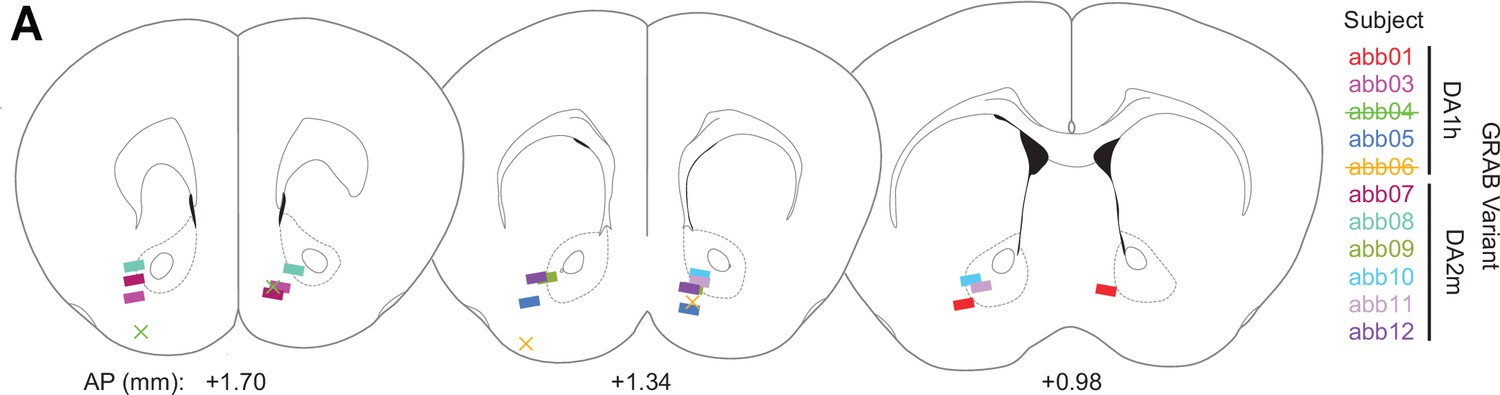
Fiber placements for fiber photometry.
(A) Position of fibers for fiber photometry experiments shown in Figure 8 (AP relative to bregma). Rectangles depict the fiber position determined by histology for mice included in the analysis, while the ‘X’ symbols depict the fiber position of two mice that were removed from the experiment for having missed lateral nucleus accumbens shell (NAcShL) placements. In the experiment, the lateralization of placements for the NAcShL and medial nucleus accumbens shell (NAcShM) were randomized across mice. For this figure, fiber positions on the left side of the diagram depict fibers targeting in the NAcShL, and fibers on the right side of the diagram depict fibers targeting in the NAcShM.
Videos
Video 1
Video of operant responding for 10% sucrose.
Video of operant responding for 10% sucrose under a fixed ratio (FR) of 1/2 turn.
Video 2
Head-fixed operant conditioning to obtain stimulation of lateral hypothalamic area GABAergic (LHAGABA) neurons or avoid stimulation of LHA glutamatergic (LHAGlut) neurons.
Videos showing responding for optogenetic stimulation of LHAGABA neurons under a positive reinforcement schedule (left) and responding for optogenetic stimulation of LHAGlut neurons under a negative reinforcement schedule (right). The LED near the center of the frame indicates when the optogenetic stimulation is turned on under positive reinforcement or when the optogenetic stimulation is turned off under negative reinforcement.
Video 3
Consumption behavior in the multi-NaCl assay under water restriction.
Video shows licking behavior during the first 25 trials of the multi-spout assay for gradients of NaCl concentrations under water restriction. Each video depicts a single 3 s trial played back at half-speed. Videos are organized to display trials from top to bottom (earlier trials on the top), and NaCl concentration from left to right (lower concentrations on the left). However, concentrations were provided in pseudorandom order.
Tables
Key resources table
| Reagent type (species) or resource | Designation | Source or reference | Identifiers | Additional information |
|---|---|---|---|---|
| Strain, strain background (Mus musculus) | Mus musculus with name C57BL/6J | https://www.jax.org/strain/000664 | RRID:IMSR_JAX:000664 | |
| Strain, strain background (Mus musculus) | Mus musculus with name Slc32a1tm2(cre)Lowl (vgat-cre) | https://www.jax.org/strain/016962 | RRID:IMSR_JAX:016962 | |
| Strain, strain background (Mus musculus) | Mus musculus with name Slc17a6tm2(cre)Lowl (vglut2-cre) | https://www.jax.org/strain/016963 | RRID:IMSR_JAX:016963 | |
| Strain, strain background (AAV5) | AAV5-EF1a-DIO-hChR2(H134R)-eYFP | UNC Vector Core | lot #: AV4313Z | |
| Strain, strain background (AAV5) | AAV5-Ef1a-DIO-mCherry | UNC Vector Core | lot #: AV4311E | |
| Strain, strain background (AAV9) | AAV9-hSyn-GRAB-DA1h | https://www.addgene.org/113050/ | Catalog #: 113050-AAV9 | lot #: v119464 |
| Strain, strain background (AAV9) | AAV9-hSyn-GRAB-DA2m | https://www.addgene.org/140553/ | Catalog #: 140553-AAV9 | lot #: v140392 |
| Software, algorithm | Sublime Text 3 | https://www.sublimetext.com/3 | ||
| Software, algorithm | Python 3.7 (Anaconda Distribution) | https://www.anaconda.com/ | ||
| Software, algorithm | R 4.0.4 | https://cran.r-project.org/ | ||
| Software, algorithm | RStudio 2022.02.3 build 492 | https://posit.co/download/rstudio-desktop/ | ||
| Software, algorithm | Arduino IDE 1.8.13 | https://www.arduino.cc/ | ||
| Software, algorithm | TinkerCad | https://www.tinkercad.com/ | ||
| Software, algorithm | OHRBETS - Analysis v1.2; | https://github.com/agordonfennell/OHRBETS/tree/main/analysis | Author: Adam Gordon-Fennell; | |
| Other | OHRBETS - Open-source hardware | https://github.com/agordonfennell/OHRBETS | 3D printing models and bill of materials | |
| Other | Optic fiber - fiber photometry | https://www.doriclenses.com/ | MFC_400/470–0.37_6mm_MF2.5_FLT | See Materials and methods |
| Other | Optic fiber - optogenetics | https://www.rwdstco.com/ | R-FOC-BL200C-39NA | See Materials and methods; item no: 907-03007-00 |
Additional files
-
Supplementary file 1
Assembly protocol.
Detailed protocol for OHRBETS (Open-Source Head-fixed Rodent Behavioral Experimental Training System) assembly.
- https://cdn.elifesciences.org/articles/86183/elife-86183-supp1-v2.pdf
-
MDAR checklist
- https://cdn.elifesciences.org/articles/86183/elife-86183-mdarchecklist1-v2.docx
-
Source data 1
Table of statistical results.
- https://cdn.elifesciences.org/articles/86183/elife-86183-data1-v2.xlsx
Download links
A two-part list of links to download the article, or parts of the article, in various formats.
Downloads (link to download the article as PDF)
Open citations (links to open the citations from this article in various online reference manager services)
Cite this article (links to download the citations from this article in formats compatible with various reference manager tools)
An open-source platform for head-fixed operant and consummatory behavior
eLife 12:e86183.
https://doi.org/10.7554/eLife.86183


