Designing optimal behavioral experiments using machine learning
- School of Informatics, University of Edinburgh, United Kingdom
- Department of Psychology, University of Edinburgh, United Kingdom
Figures
Figure 1
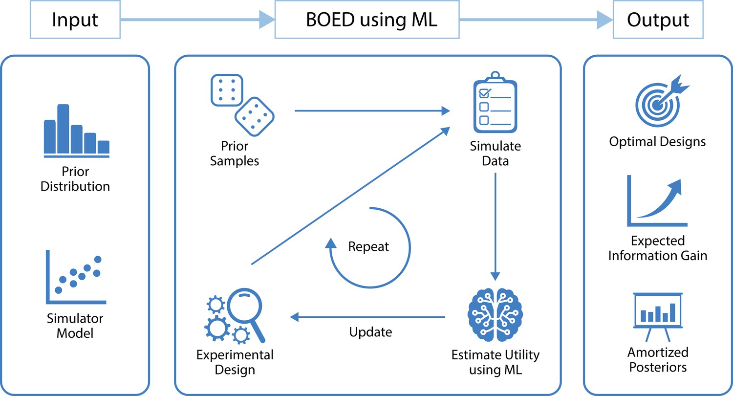
A high level overview of our approach that uses machine learning (ML) to optimize the design of experiments.
The inputs to our method are a model from which we can simulate data and a prior distribution over the model parameters. Our method starts by drawing a set of samples from the prior and initializing an experimental design. These are used to simulate artificial data using the simulator model. We then use ML to estimate the expected information gain of those data, which is used as a metric to search over the design space. Finally, this is repeated until convergence of the expected information gain. The outputs of our method are optimal experimental designs, an estimate of the expected information gain when performing the experiment and an amortized posterior distribution, which can be used to cheaply compute approximate posterior distributions once real-world data are observed. Other useful by-products of our method include a set of approximate sufficient summary statistics and a fitted utility surface of the expected information gain.
Box 1—figure 1
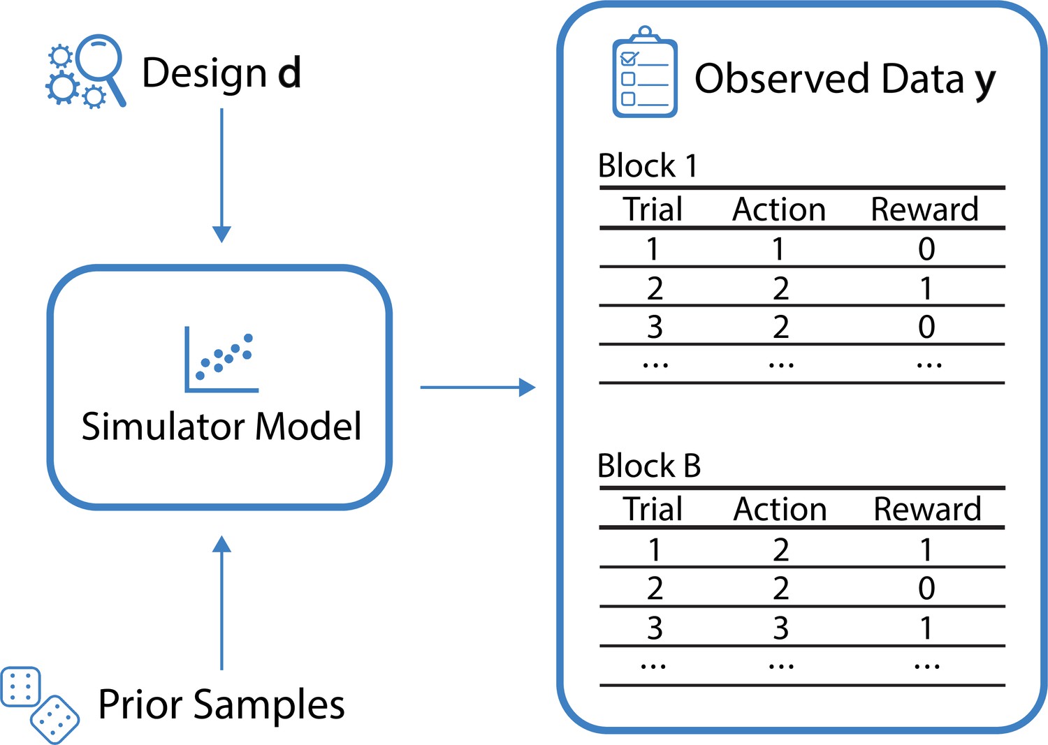
Schematic of the data-generating process for the example of multi-armed bandit tasks.
For a given design d (here the reward probabilities associated with the bandit arms in each individual block) and a sample from the prior over the model parameters , the simulator generates observed data , corresponding to the actions and rewards from blocks.
Box 4—figure 1
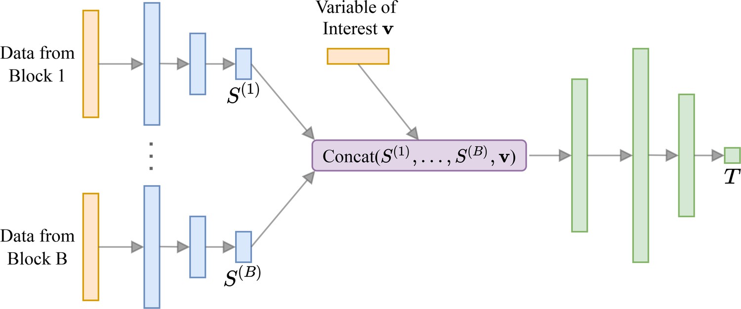
Neural network architecture for behavioral experiments.
For each block of data we have a small sub-network (shown in blue) that outputs summary statistics S. These are concatenated with the variable of interest (e.g. corresponding to a model indicator for model discrimination tasks) and passed to a larger neural network (shown in green). Box 4—figure 1 has been adapted from Figure 1 in Valentin et al., 2021.
Box 5—figure 1
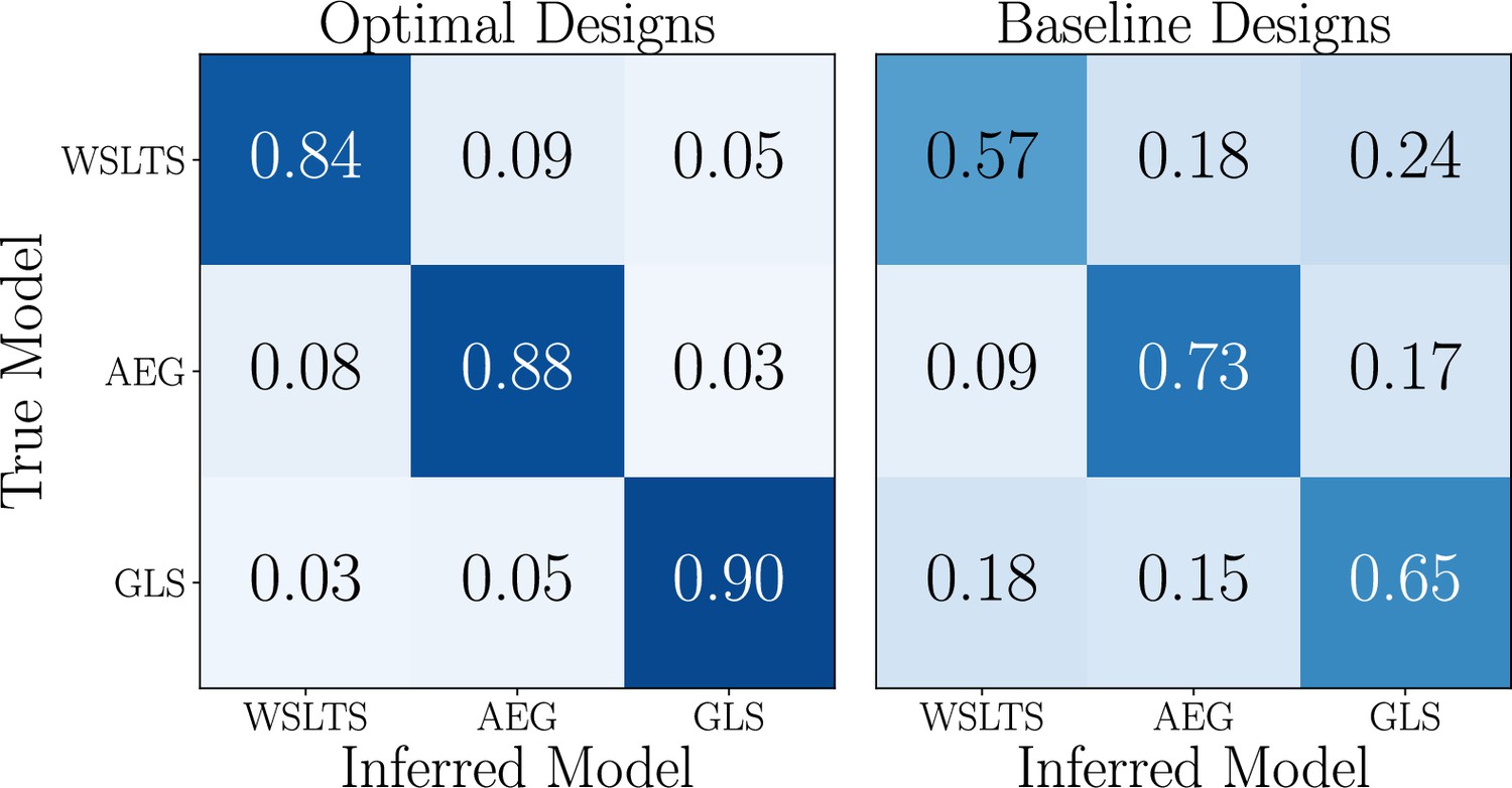
Simulation study results for the model discrimination task, showing the confusion matrices of the inferred behavioral models, for optimal (left) and baseline (right) designs.
Box 5—figure 1 has been adapted from Figure 2 in Valentin et al., 2021.
Box 6—figure 1
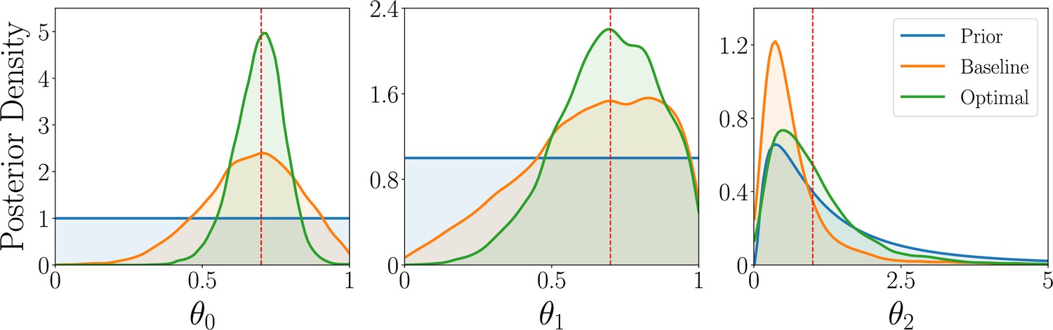
Simulation study results for the parameter estimation task of the WSLTS model, showing the marginal posterior distributions of the three WSLTS model parameters for optimal (green) and baseline (orange) designs, averaged over 1,000 simulated observations.
The ground-truth parameter values were chosen in accordance with previous work on simpler versions of the WSLTS model (Zhang and Lee, 2010) and as plausible population values for the posterior reshaping parameter.
Box 8—figure 1
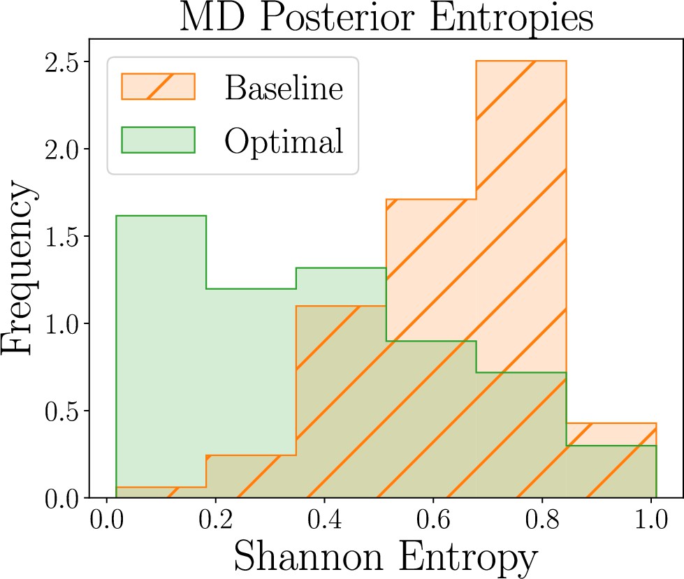
Human-participant study results for the model discrimination (MD) task, showing thedistribution of posterior Shannon entropies obtained for optimal (green) and baseline (orange)designs (lower is better).
Box 8—figure 2

Human-participant study results for the parameter estimation (PE) task of the AEG model,showing the distribution of posterior differential entropies obtained for optimal (green) and baseline(orange) designs (lower is better).
Box 9—figure 1
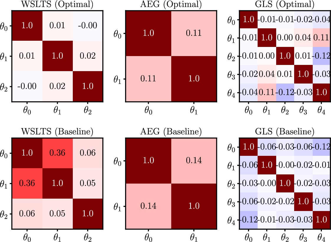
Human-participant study average linear correlations in the posterior distribution of model parameters for all models in the parameter estimation task, and for both optimal (top) and baseline (bottom) designs.
Appendix 5—figure 1

Screenshot of bandit task that participants completed in online experiments.
Appendix 5—figure 2
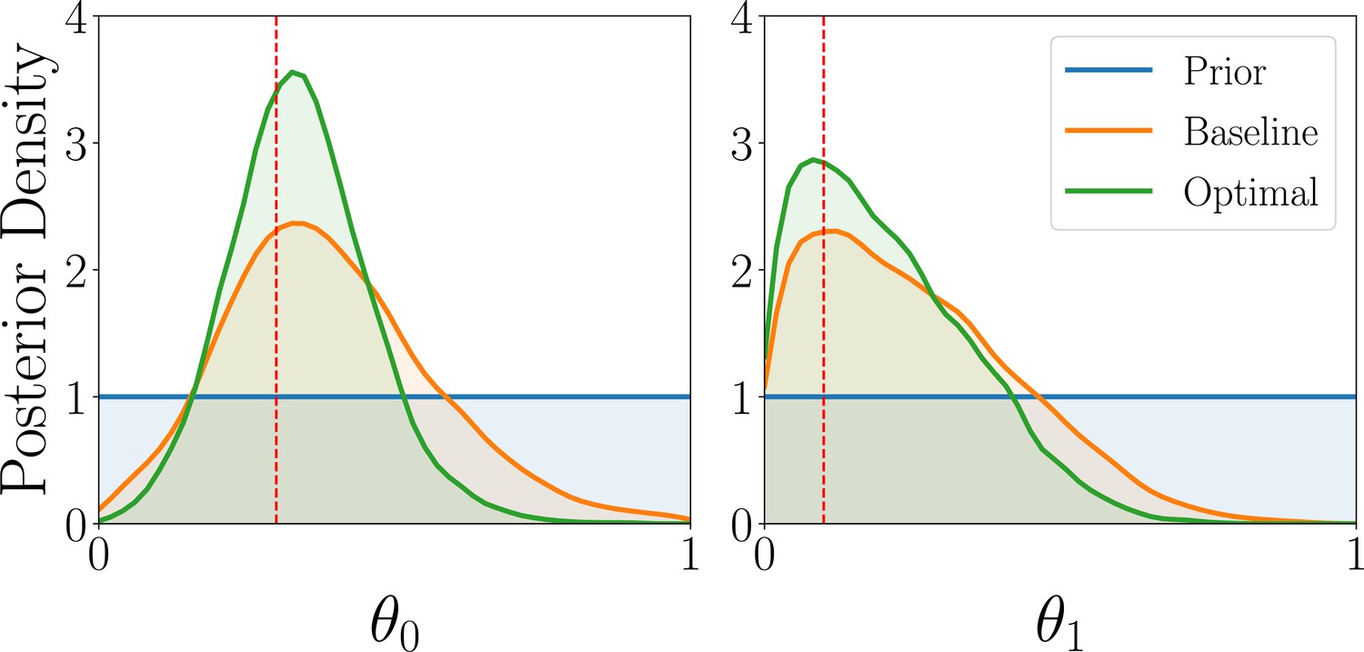
Results for the parameter estimation task of the AEG model, showing the marginal posterior distributions of the three AEG model parameters for optimal (green) and baseline (orange) designs, averaged over 1000 observations.
Appendix 5—figure 3
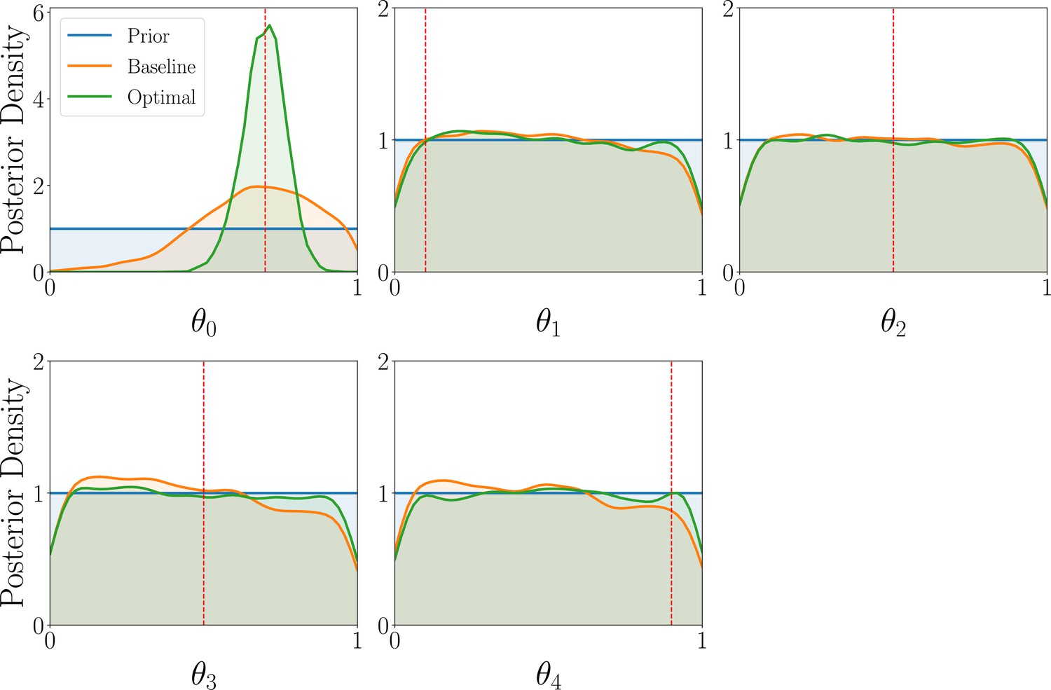
Results for the parameter estimation task of the GLS model, showing the marginal posterior distributions of the three GLS model parameters for optimal (green) and baseline (orange) designs, averaged over 1000 observations.
Appendix 5—figure 4
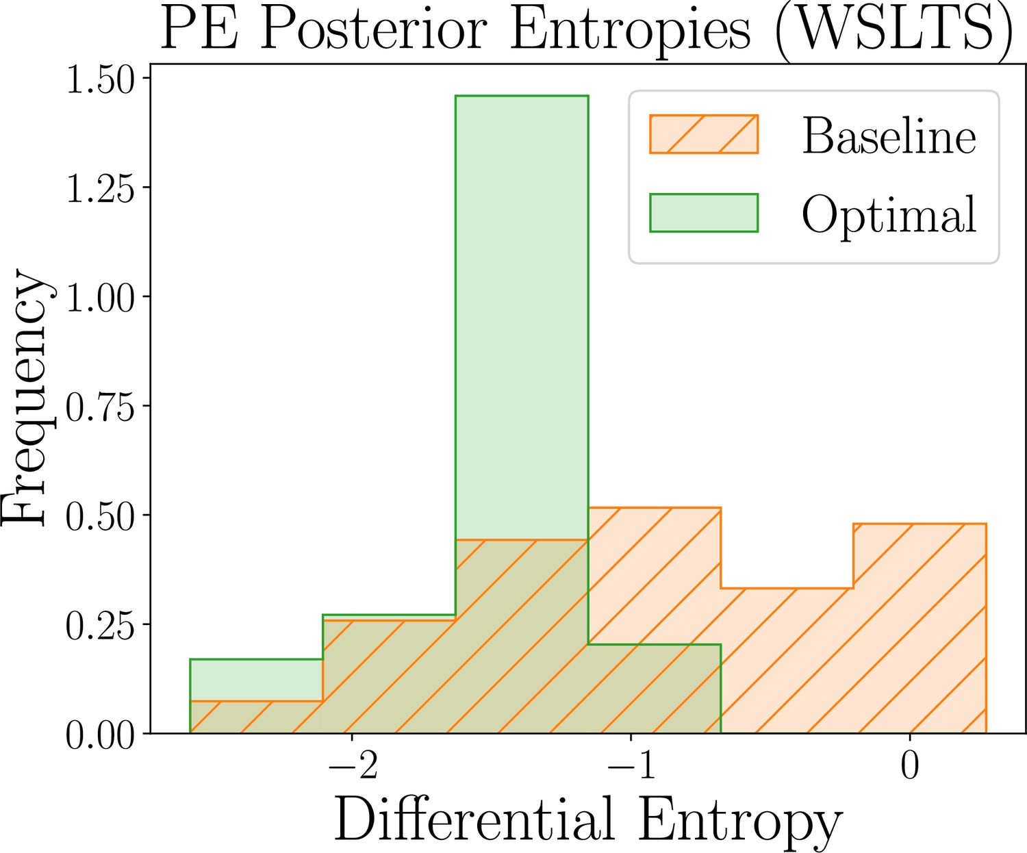
Results for the parameter estimation task of the WSLTS model, showing the distribution of posterior differential entropies obtained for optimal (green) and baseline (orange) designs (lower is better).
Appendix 5—figure 5
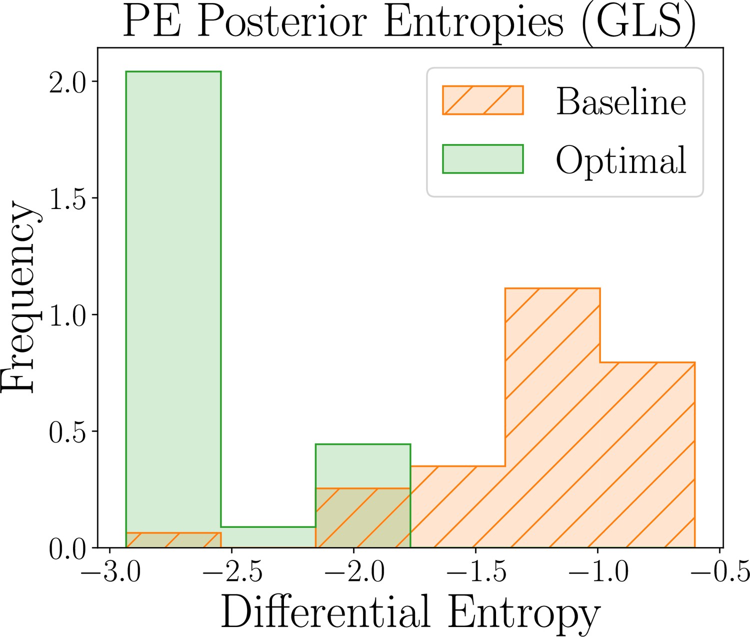
Results for the parameter estimation task of the GLS model, showing the distribution of posterior differential entropies obtained for optimal (green) and baseline (orange) designs (lower is better).
Appendix 5—figure 6
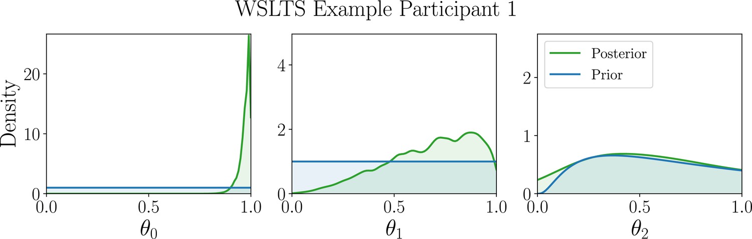
Marginal posterior distributions (green) of the WSLTS model parameters for example participant 1.
Appendix 5—figure 7
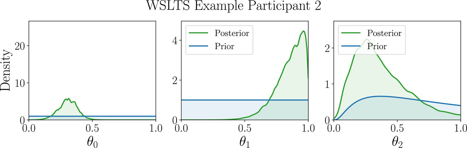
Marginal posterior distributions (green) of the WSLTS model parameters for example participant 2.
Appendix 5—figure 8
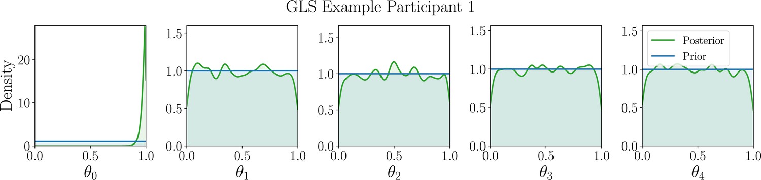
Marginal posterior distributions (green) of the GLS model parameters for example participant 1.
Appendix 5—figure 9
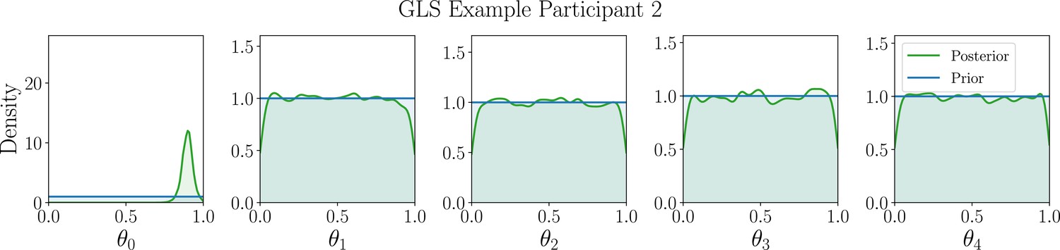
Marginal posterior distributions (green) of the GLS model parameters for example participant 2.
Appendix 6—figure 1
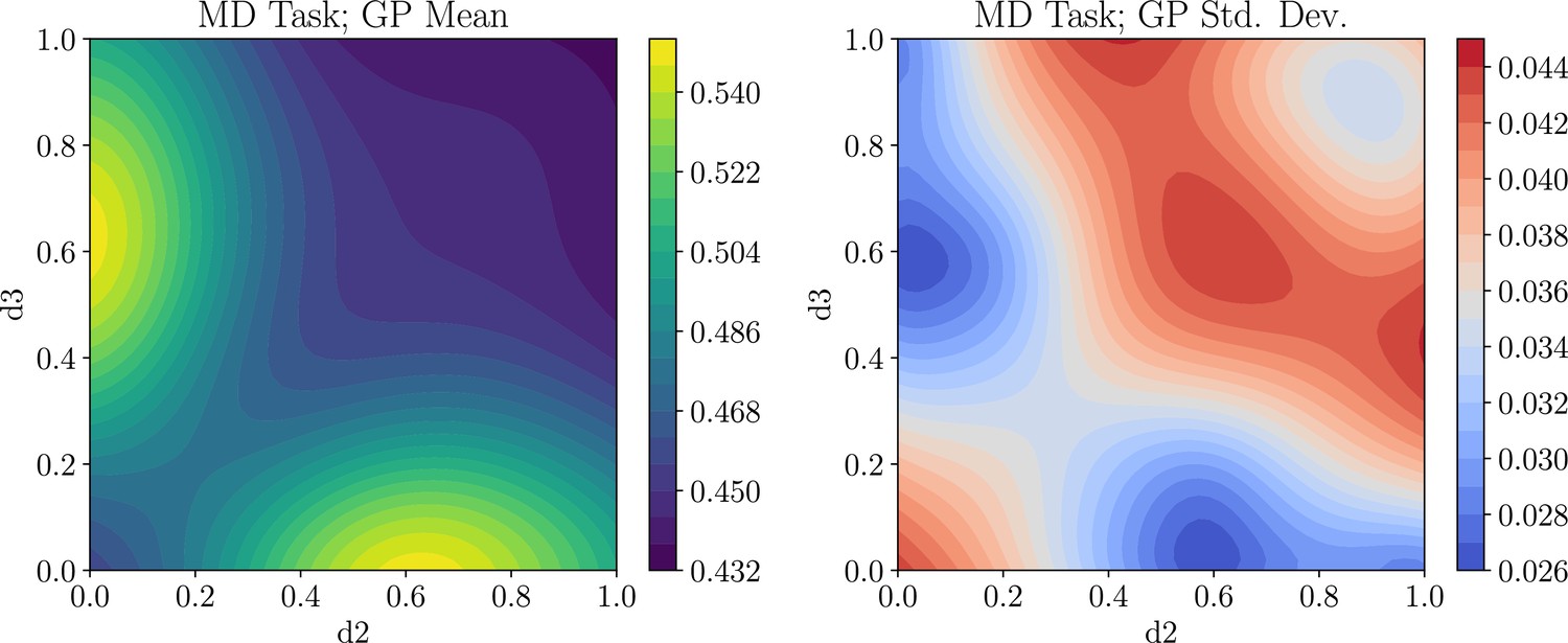
Example of how to explore the high-dimensional utility function for the model discrimination (MD) task, by slicing the Gaussian process (GP) learned during the design optimization step.
The left plot shows the mean of the GP and the right plot shows the standard deviation of the GP. Shown is the slice corresponding to the design, which contains the global optimum.
Appendix 7—figure 1
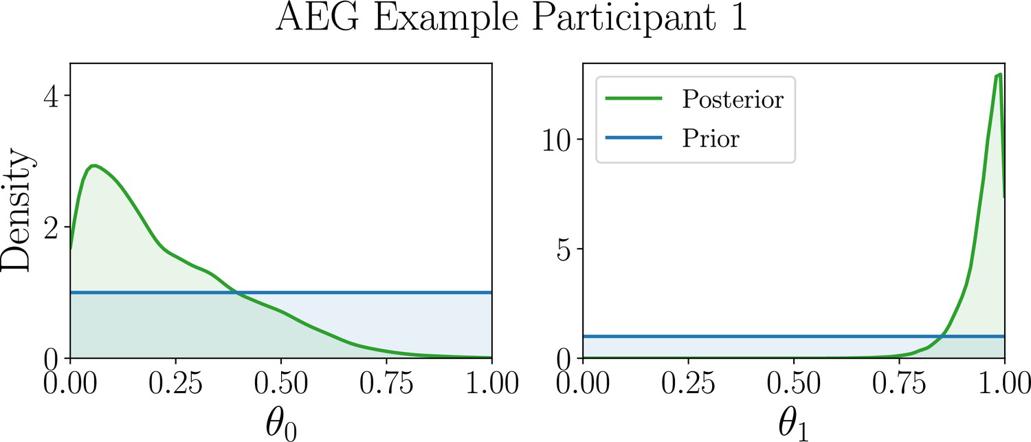
Inferred marginal posterior model parameters for human participants best described by the AEG model.
Marginal posterior distributions (green) of the AEG model parameters for example participant 1.
Appendix 7—figure 2
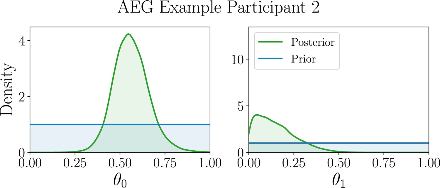
Posterior distribution (green) of the AEG model parameters for example participant 2.
Appendix 7—figure 3
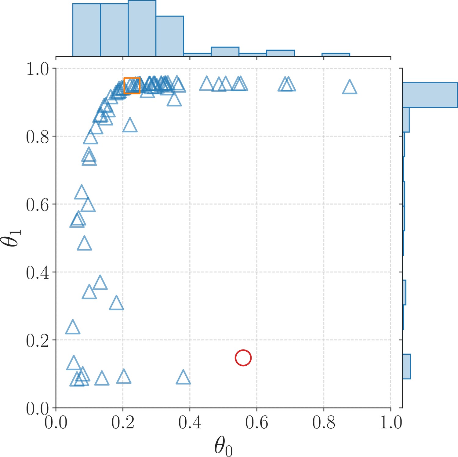
Mean values of the parameter posterior distributions for each of the 75 participants best described by the AEG model; the square and circle markers represent example participants 1 and 2, respectively.
Tables
Appendix 6—table 1
A ranking of local design optima for the model discrimination task.
Shown are the rank, the mutual information (MI) estimate computed via the Gaussian process (GP) mean, and the locally optimal designs. Note that, for this task, the designs for the first bandit arm were and for the second bandit arm. The 5 unique optima were obtained by running stochastic gradient ascent on the GP mean with 20 restarts.
| Rank of Optimum | MI | ||||||
|---|---|---|---|---|---|---|---|
| 1 | 0.672 | 0.000 | 0.000 | 0.607 | 1.000 | 1.000 | 0.000 |
| 2 | 0.526 | 1.000 | 0.006 | 1.000 | 0.140 | 0.266 | 0.528 |
| 3 | 0.485 | 0.000 | 1.000 | 0.774 | 0.275 | 0.399 | 0.630 |
| 4 | 0.479 | 0.683 | 0.775 | 0.000 | 0.216 | 0.717 | 0.128 |
| 5 | 0.475 | 0.009 | 0.710 | 0.583 | 0.842 | 0.000 | 0.109 |
Download links
A two-part list of links to download the article, or parts of the article, in various formats.
Downloads (link to download the article as PDF)
Open citations (links to open the citations from this article in various online reference manager services)
Cite this article (links to download the citations from this article in formats compatible with various reference manager tools)
Designing optimal behavioral experiments using machine learning
eLife 13:e86224.
https://doi.org/10.7554/eLife.86224


