Hydrodynamics and multiscale order in confluent epithelia
- Instituut-Lorentz, Leiden University, Netherlands
Figures
Figure 1
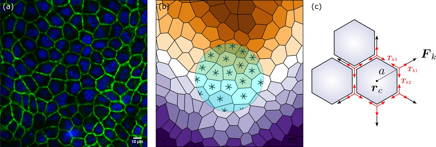
Epithelia and hexanematic order.
(a) Example of multiscale hexanematic order in an in vitro layer of Madin–Darby canine kidney (MDCK) cells (b) and its computer-constructed segmentation. Both panels are adapted from Figure 3 of Armengol-Collado et al., 2023. The six-legged stars in the shaded region denote the sixfold orientation of the cells obtained using the approach summarized in Methods. The colored stripes mark the configuration of the nematic director at the length scale of the light-blue disk. (c) Schematic representation of the sixfold symmetric force complexion exerted by cells. The red arrows indicate the structure of the contractile forces acting within the cellular junctions.
Figure 2
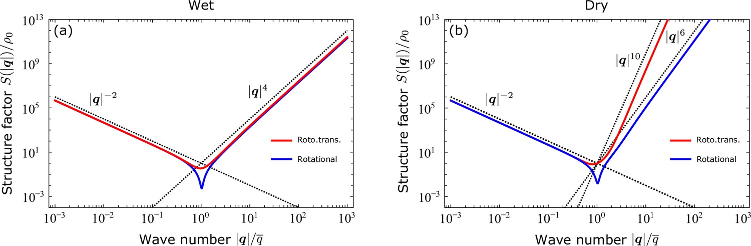
Structure factor obtained from the analytical solutions of the linearized hydrodynamic equations in the presence of two different noise fields: purely rotational (blue) and rototranslational (red).
The full analytical expression of is given in Methods, together with a derivation of the exact asymptotic expansions of Equation (8). (a) As long as viscous dissipation takes place (i.e. ‘wet’ regime), in the limit , irrespective of the type of noise. (b) On the other hand, when friction is the sole momentum dissipation mechanism at play (‘dry’ regime), in case of rotational noise and when noise is both rotational and translational. In both panels, the wave number is rescaled by , with and and as defined in Equation (7).
Figure 3
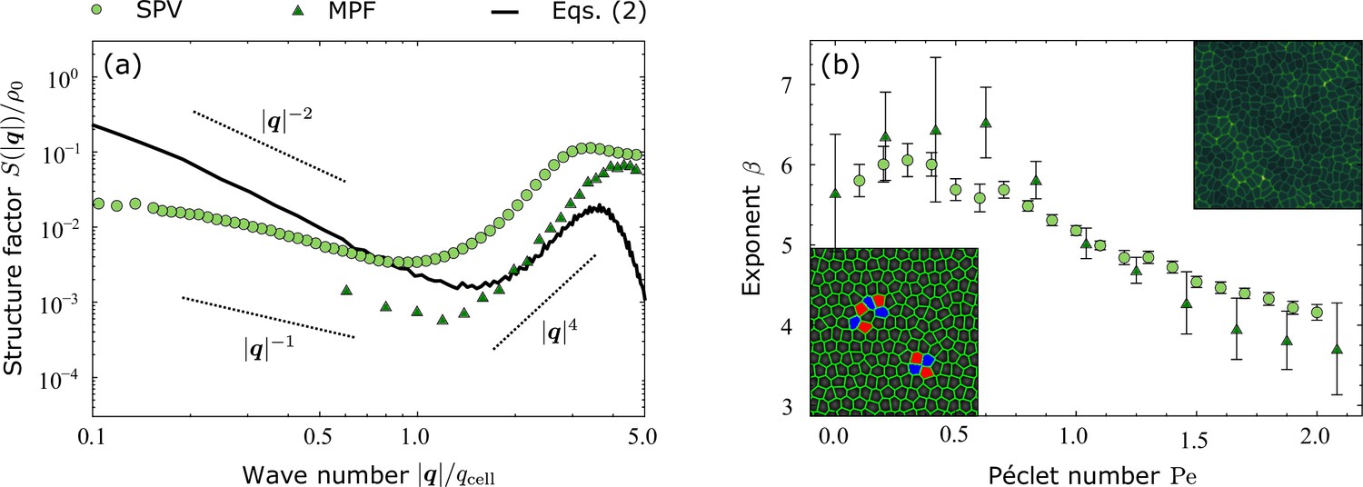
Density fluctuations in model epithelia.
(a) Structure factor of model-epithelia calculated from a numerical integration of Equation 2a (black line) and from simulations of two different cell-resolved models: i.e. the self-propelled Voronoi model (SPV, red) and the multiphase field (MPF) model (blue), for a particular choice of parameters. The dashed diagonal lines mark the scaling regimes obtained analytically at the linear order, Equation (8), and the wave number is rescaled by , where is the grid size used by the Lattice Boltzmann integrator (see Methods for details). (b) The exponent , as defined in Equation (8), versus the Péclet number , reflecting the persistence of directed cellular motion in front of diffusion. Error bars calculated as standard error over $n=250$ configurations for both the SPV and the MPF models. Insets: typical configurations of the SPV (bottom left) and MPF (top right) models.
Figure 4
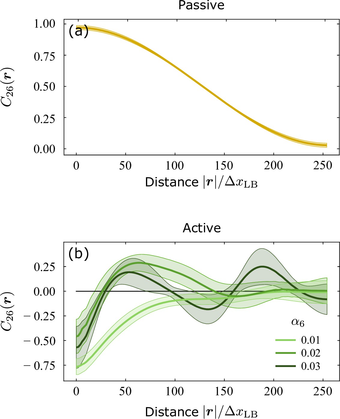
Cross-correlation function , as defined in Equation 9, obtained from a numerical integration of Equation 2a augmented with rotational noise.
(a) In the passive case, when and , the correlation function decays with at a rate i.e. lower at short distances, where the dynamics of the hexatic and nematic orientations is dominated by fluctuations, and larger at long distances, where the orientations are ‘locked’ in a parallel configuration, or tilted by with respect to each other. (b) In the active case, conversely, the cross-correlation function has a damped oscillatory behavior. Consistently with Equation (7) and the related discussion, the range of the oscillations, corresponding to the distance at which these are fully damped, increases with the hexatic activity , indicating an enhancement of hexatic order at larger length scales. Shaded region corresponding to the standard deviation of configurations. Distance is expressed in terms of the grid size used by the Lattice Boltzmann integrator (see Methods for details).
Figure 5
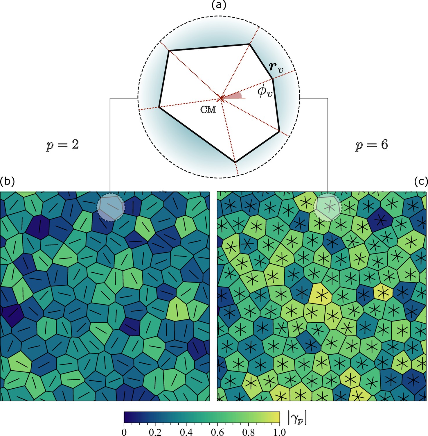
Nematic and hexatic shape function.
(a) Irregular polygonal cell with a red cross marking its center of mass and and the radial vector and the angle to one of the six vertices, respectively. (b) and (c) show the same tessellation of the plane with cells of different shapes and the shape analysis using the function in Equation 10 for the nematic () and hexatic () case. Rods and stars are oriented according to the phase of and the color corresponds to its magnitude.
Figure 6
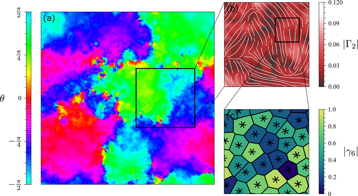
Hexanematic symmetry of Voronoi model.
(a) Coarse-grained nematic orientation obtained from averaging the local shape of cells over domains of size , with the average size of individual cells. Regions with the same color represent domains of coherent nematic orientation. (b) Part of the system where we use to characterize the nematic phase. Solid lines represent the nematic director and the color inditicates the magnitude of the nematic shape function. (c) Voronoi cell structure of a region where the nematic field is uniform. Polygons are colored according to and the stars are oriented according to .
Download links
A two-part list of links to download the article, or parts of the article, in various formats.
Downloads (link to download the article as PDF)
Open citations (links to open the citations from this article in various online reference manager services)
Cite this article (links to download the citations from this article in formats compatible with various reference manager tools)
Hydrodynamics and multiscale order in confluent epithelia
eLife 13:e86400.
https://doi.org/10.7554/eLife.86400


