Variability of visual field maps in human early extrastriate cortex challenges the canonical model of organization of V2 and V3
- School of Psychology, The University of Queensland, Australia
- Queensland Brain Institute, The University of Queensland, Australia
- School of Electrical Engineering and Computer Science, The University of Queensland, Australia
- Department of Physiology, Monash University, Australia
- Neuroscience Program, Biomedicine Discovery Institute; Monash University, Australia
- Department of Electrical and Computer Systems Engineering, Monash University, Australia
- Queensland Digital Health Centre, The University of Queensland, Australia
Figures
Figure 1 with 1 supplement
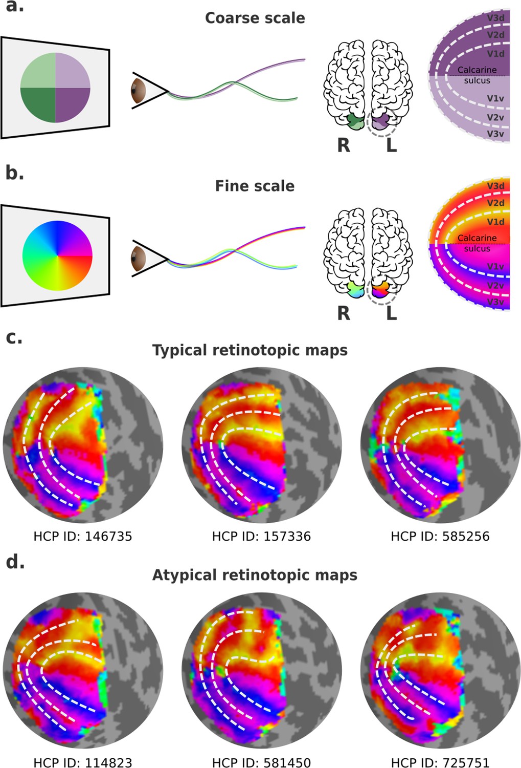
Visual field mapping in the human early visual cortex.
(a) Coarse scale visual field mapping in the early visual cortex. The left (L) hemisphere maps the right visual field, and the right (R) hemisphere maps the left visual field. The dorsal portion of early visual areas maps the lower hemifield, and the ventral portion the upper field. (b) Fine scale visual field mapping with visual field maps represented in polar angles (0–360°). In this model, the vertical (90° or 270°) and horizontal meridians (0° for the left and 180° for the right hemispheres) delineate boundaries between visual areas. (c) Three ‘classical’ polar angle maps, obtained from the left hemispheres of three individuals in the Human Connectome Project (HCP) retinotopy dataset, which conform to the traditional model. (d) Three polar angle maps that deviate from this pattern, obtained from left hemispheres of three other individuals in the HCP retinotopy dataset. In the latter, the isopolar bands representing the anterior borders of dorsal V3 (V3d) and dorsal V2 (V2d) do not follow the proposed borders of V2 and V3 (dashed lines).
Figure 1—figure supplement 1
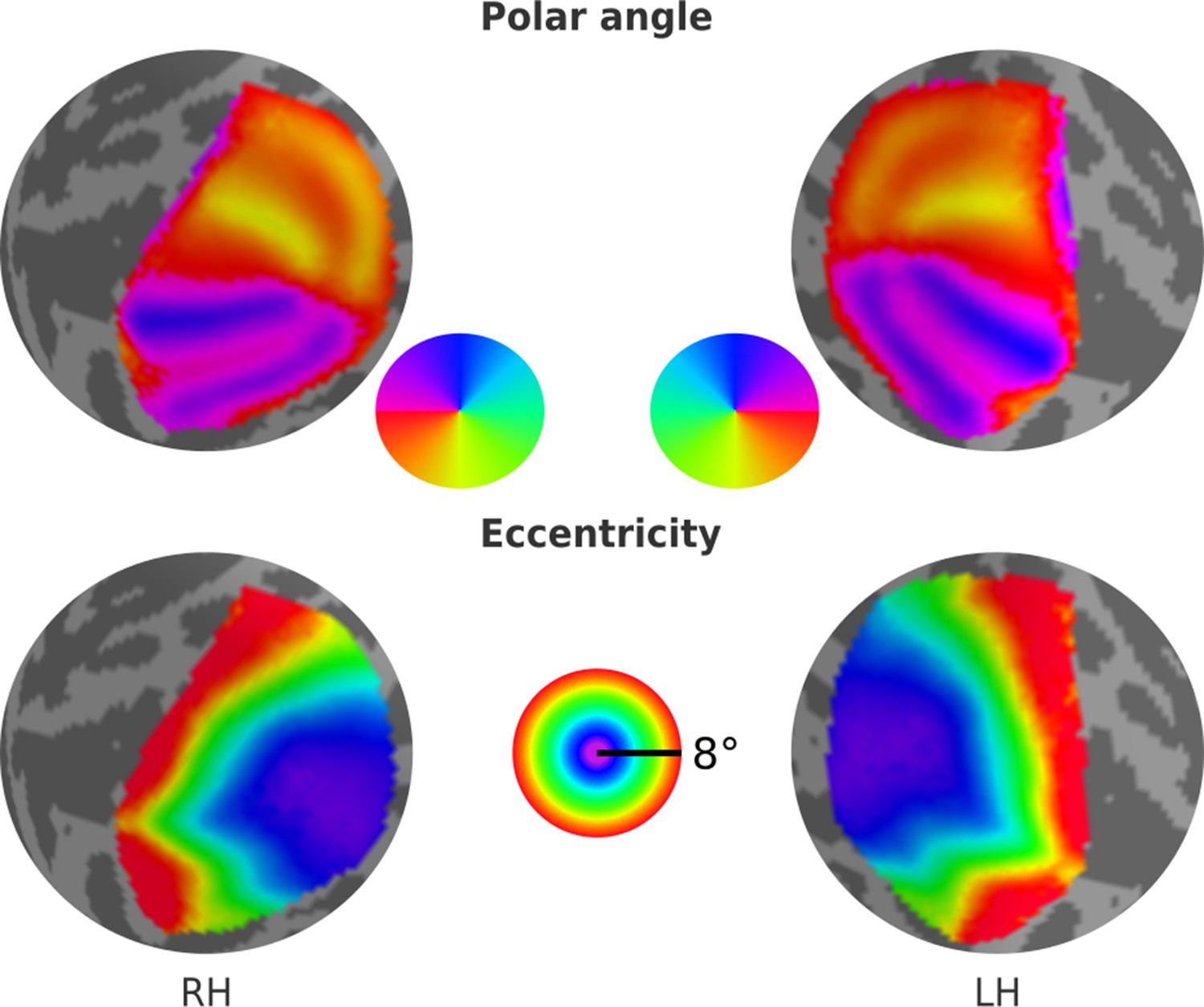
Average retinotopic maps across all 181 individuals from the Human Connectome Project (HCP) retinotopy dataset for both left (LH) and right (RH) hemispheres.
Figure 2
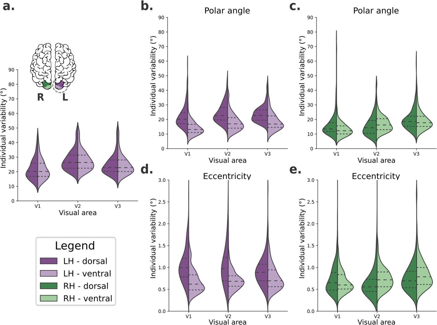
Individual variability in visual field maps of early visual areas.
(a) Hypothetical diagram of symmetrical distributions of individual variability across visual areas. The center and right columns illustrate empirical distributions of individual variability of polar angle (b, c) and eccentricity (d, e) maps for both dorsal (dark shades) and ventral (lighter shades) portions of early visual areas in left (purple) and right (green) hemispheres.
Figure 3 with 1 supplement
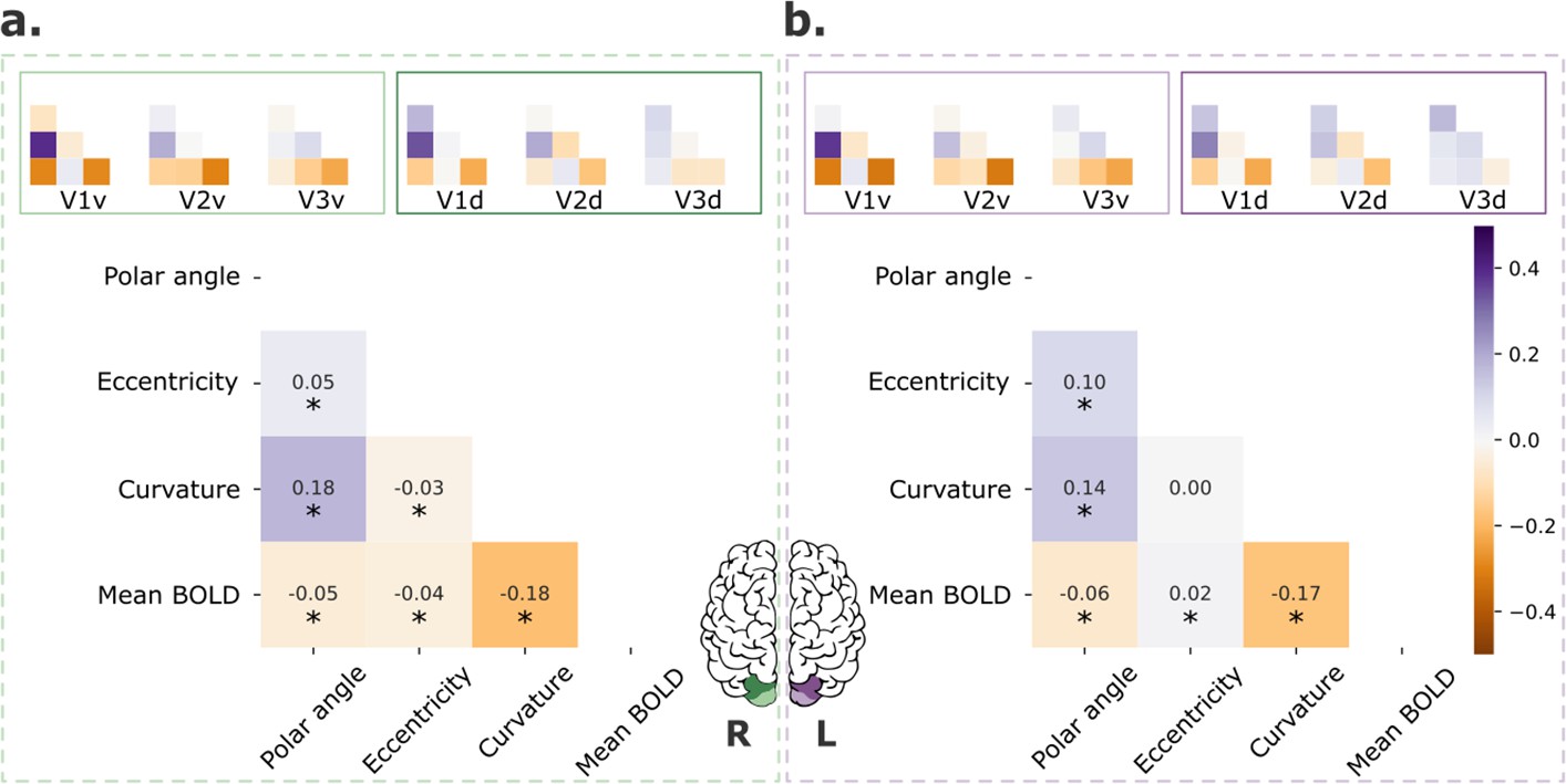
Retinotopic maps correlation with covariates.
Pair-wise correlations among polar angle, eccentricity, curvature, and normalized mean BOLD signal for early visual areas (V1–3; main plot) and each visual area separately (inset plots), for both left (a) and right (b) hemispheres. Polar angle maps were converted such that 0° corresponds to the horizontal meridian and 90° corresponds to the upper and lower vertical meridians (Kurzawski et al., 2022). Finally, data were concatenated across all participants (n = 181). *p < 0.001.
Figure 3—figure supplement 1
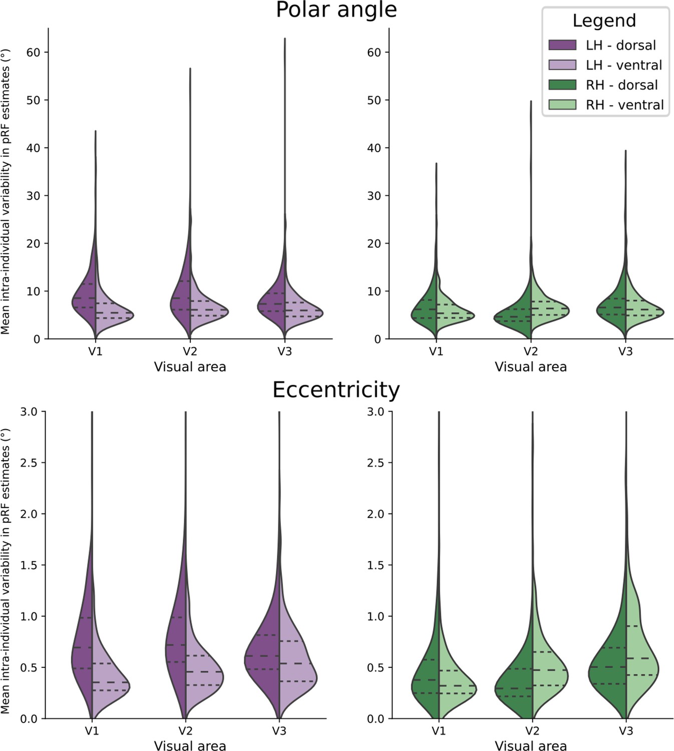
Intra-individual variability in visual field maps of early visual areas.
Empirical distributions of intra-individual variability of polar angle (top) and eccentricity (bottom) maps for both dorsal (dark shades) and ventral (lighter shades) portions of early visual areas in the left (purple) and right (green) hemispheres. The intra-individual variability is the difference in pRF estimates from two pRF model fits; each used half of the retinotopic mapping data (see Supplementary file 7 for more information).
Figure 4 with 2 supplements
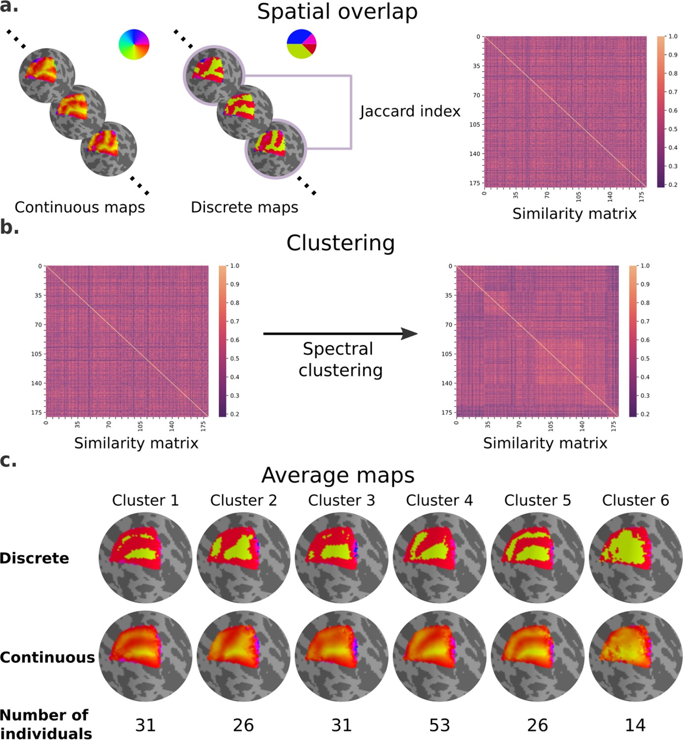
Clusters of retinotopic organization in the dorsal portion of early visual cortex.
(a) Continuous polar angle maps were converted into discrete maps, such that each vertex would be categorized into one out of four possible labels. Spatial overlap between discrete maps was estimated using the Jaccard similarity coefficient from all possible pairs of individuals, resulting in a 181 × 181 similarity matrix. (b) Then, we applied a spectral clustering algorithm – setting the number of clusters to 6. (c) An average map (discrete and continuous) was calculated for each cluster by averaging the continuous polar angle maps across all individuals within each cluster.
Figure 4—figure supplement 1

Clusters of eccentricity maps of the dorsal portion of early visual cortex.
An average continuous map was calculated for each cluster by averaging the continuous eccentricity maps across all individuals within each cluster.
Figure 4—figure supplement 2
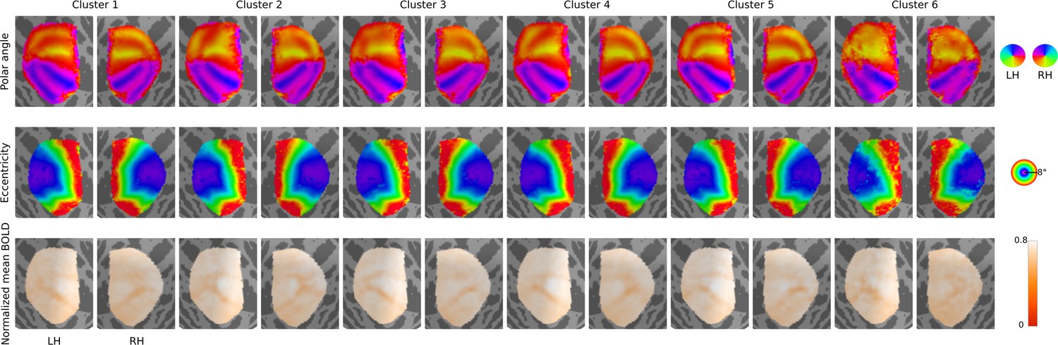
Average polar angle, eccentricity, and normalized mean BOLD signal maps from each cluster and hemisphere.
Average continuous polar angle, eccentricity, and normalized mean BOLD signal maps were calculated for each cluster by averaging the continuous maps across all individuals within each cluster. As in the manuscript, the cluster assignment was based on the clustering analysis with polar angle maps from the dorsal portion of the early visual cortex and left hemisphere.
Figure 5 with 6 supplements
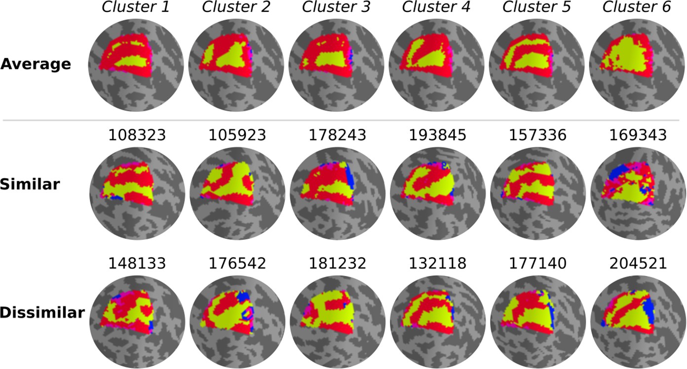
Qualitative evaluation of clusters.
Average cluster maps are shown in the top row. The middle row shows examples of maps from each cluster with a similar retinotopic organization to the corresponding average map. Finally, in the bottom row, examples of those with dissimilar organizations are shown.
Figure 5—figure supplement 1

Nine randomly selected polar angle maps within cluster 1.
The average discrete map of cluster 1 is shown.
Figure 5—figure supplement 2

Individual polar angle maps within cluster 2.
The average discrete map of cluster 2 is shown. All individuals’ polar angle maps within cluster 2 (total of 26 individuals) are shown for qualitative examination.
Figure 5—figure supplement 3
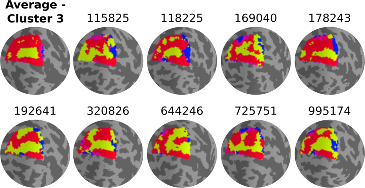
Nine randomly selected polar angle maps within cluster 3.
The average discrete map of cluster 3 is shown.
Figure 5—figure supplement 4

Nine randomly selected polar angle maps within cluster 4.
The average discrete map of cluster 4 is shown.
Figure 5—figure supplement 5
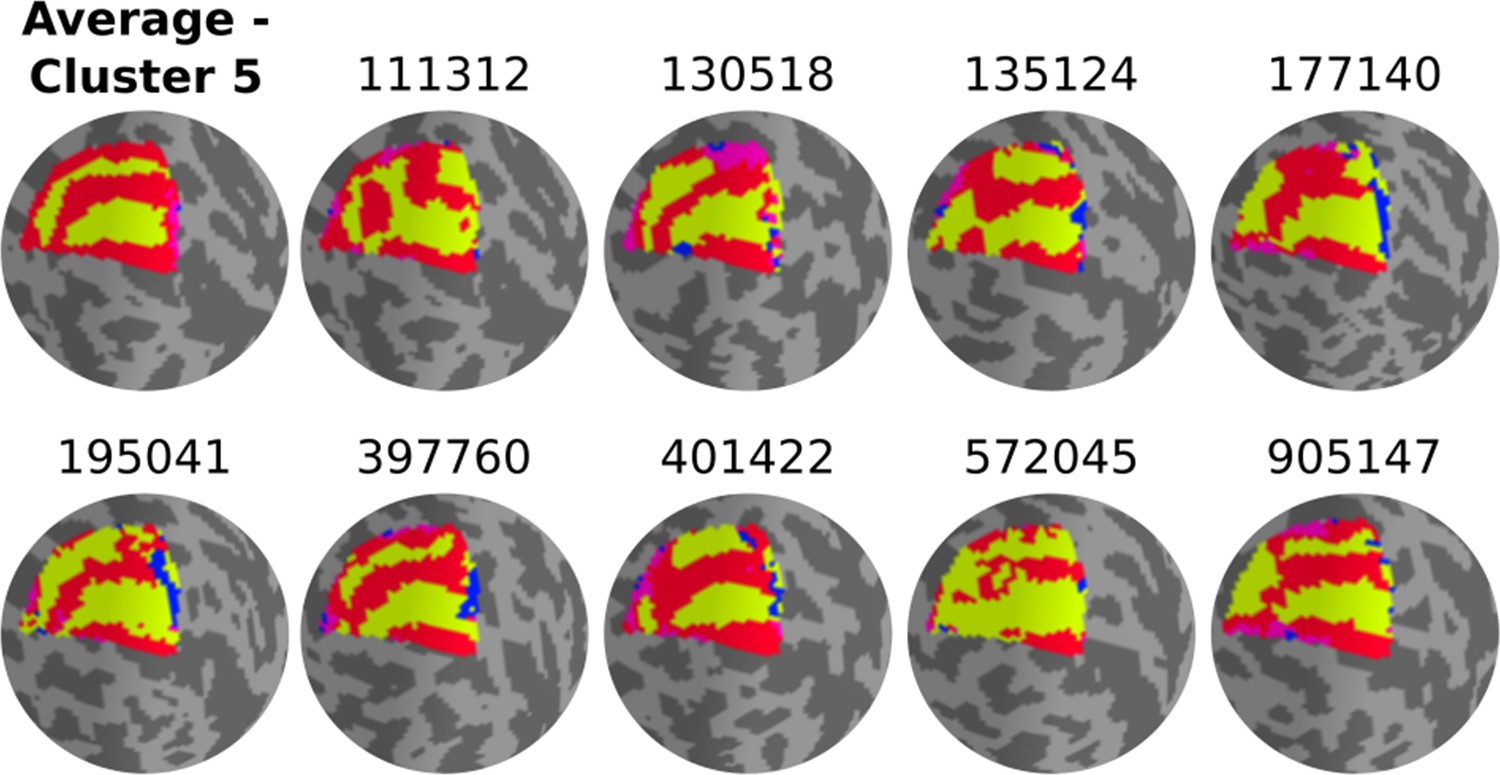
Nine randomly selected polar angle maps within cluster 5.
The average discrete map of cluster 5 is shown.
Figure 5—figure supplement 6

Nine randomly selected polar angle maps within cluster 6.
The average discrete map of cluster 6 is shown.
Figure 6
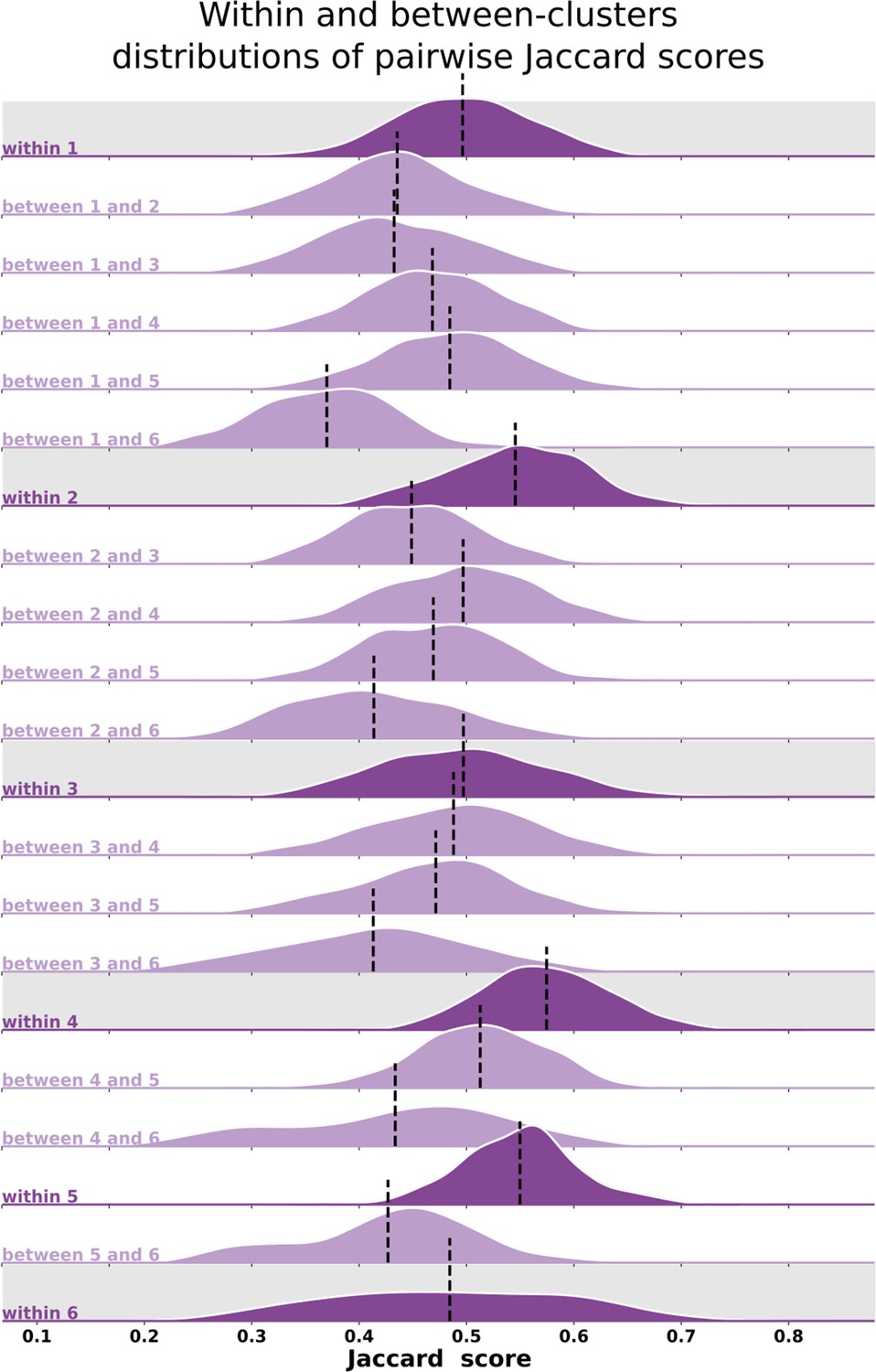
Distributions of pair-wise Jaccard scores.
Within- and between-cluster distribution of Jaccard scores across all pairs of individuals. Within-cluster distributions are highlighted in gray. Between-cluster distributions are the same regardless of the order of the clusters, that is, the Jaccard score distribution between clusters 1 and 2 (between 1 and 2) is the same as the one between clusters 2 and 1. Black vertical lines indicate distributions’ means.
Figure 7 with 1 supplement
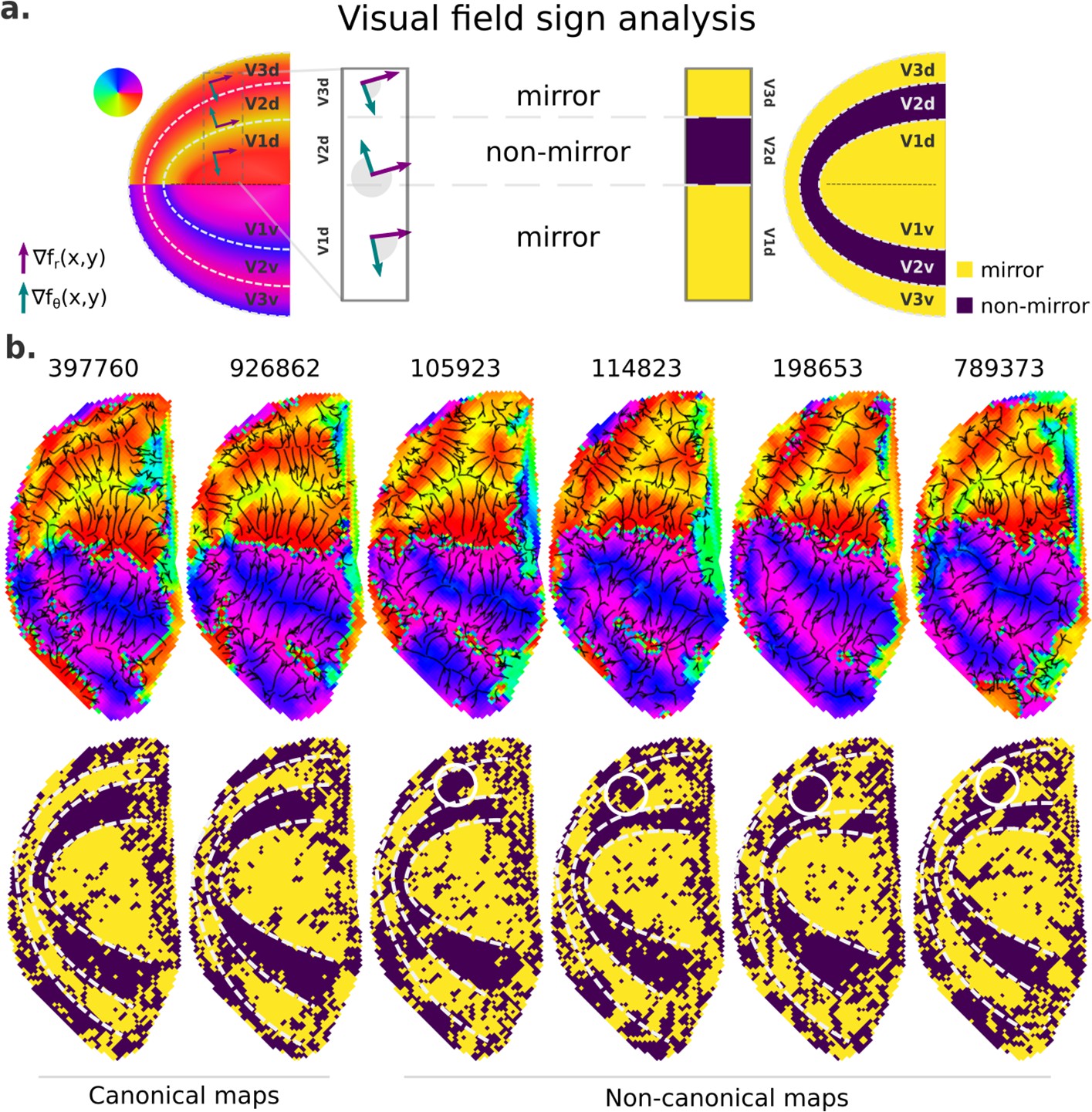
Visual field sign analysis for delineating visual areas.
(a) The visual field sign analysis (Sereno et al., 1995; Sereno et al., 1994) combines polar angle and eccentricity maps (not shown) into a unique representation of the visual field as either a non-mirror-image (like V2) or a mirror-image (like V1) representation of the retina. This analysis consists of determining the angle between the polar angle and eccentricity maps’ gradient vectors, respectively, the green and purple vectors, at each cortical coordinate. If the angle between the gradient vectors is between 0 and π, by convention, the cortical patch is a mirror-image representation of the retina; otherwise, it is a non-mirror-image. (b) Six examples of left hemisphere polar angle maps with canonical (on the left) and non-canonical (on the right) representations in the dorsal portion of early visual cortex are shown (top row). Polar angle gradients are shown in a ‘streamline’ representation to highlight reversals in the progression of the polar angle values. Their respective visual field sign representation (bottom row) is also shown. While it was unclear how to delineate boundaries in the dorsal portion of polar angle maps in those participants with non-canonical maps, the visual field sign representation reveals that the area identified as dorsal V3 shows a discontinuity in the canonical mirror-image representation (solid white circles).
Figure 7—figure supplement 1

Visual field sign analysis for delineating visual areas.
Five more examples of left hemisphere polar angle maps with unusual Y-shaped lower vertical representations are shown in the top half. Polar angle gradients are shown in a ‘streamline’ representation (first row) with their respective visual field sign representation (second row). In the bottom half are five other examples of polar angle maps with a truncated V3 boundary, indicating that dorsal V3 does not cover the entire quarter visual field (i.e., from 360° to 270°). Despite that, the visual field sign representation does not show discontinuity in the typical mirror-image representation of dorsal V3.
Tables
Table 1
Fixed effects parameter estimates for the linear mixed-effect model of individual variability of polar angle maps.
| Polar angle | ||||||||
|---|---|---|---|---|---|---|---|---|
| 95% CI | ||||||||
| Names | Effect | Estimate | SE | Lower | Upper | df | t | p |
| Intercept | Intercept | 18.58 | 0.30 | 17.99 | 19.17 | 180 | 61.86 | <0.001 |
| Hemisphere | RH–LH | −3.35 | 0.32 | −3.97 | −2.72 | 181 | −10.47 | <0.001 |
| Visual area (1) | V2–V1 | 2.38 | 0.29 | 1.81 | 2.95 | 210 | 8.21 | <0.001 |
| Visual area (2) | V3–V1 | 3.99 | 0.32 | 3.36 | 4.61 | 187 | 12.54 | <0.001 |
| Portion | Ventral–dorsal | −3.30 | 0.29 | −3.86 | −2.74 | 181 | −11.50 | <0.001 |
-
SE – standard error; CI – confidence interval.
Table 2
Fixed effects parameter estimates for the linear mixed-effect model of individual variability of eccentricity maps.
| Eccentricity | ||||||||
|---|---|---|---|---|---|---|---|---|
| 95% CI | ||||||||
| Names | Effect | Estimate | SE | Lower | Upper | df | t | p |
| Intercept | Intercept | 0.81 | 0.02 | 0.77 | 0.85 | 180 | 41.86 | <0.001 |
| Hemisphere | RH–LH | −0.14 | 0.01 | −0.16 | −0.11 | 181 | −10.91 | <0.001 |
| Visual area (1) | V2–V1 | 0.01 | 0.01 | −0.01 | 0.04 | 402 | 0.98 | 0.326 |
| Visual area (2) | V3–V1 | 0.05 | 0.01 | 0.02 | 0.08 | 182 | 3.24 | 0.001 |
| Portion | Ventral–dorsal | −0.13 | 0.03 | −0.18 | −0.07 | 180 | −4.64 | <0.001 |
-
SE – standard error; CI – confidence interval.
Table 3
Fixed effects parameter estimates for the linear mixed-effects model of individual variability of polar angle maps using covariates.
The covariates included in the model were intra-individual variability in pRF estimates, and individual variability in curvature and the mean BOLD signal.
| Polar angle | ||||||||
|---|---|---|---|---|---|---|---|---|
| 95% CI | ||||||||
| Names | Effect | Estimate | SE | Lower | Upper | df | t | p |
| Intercept | Intercept | 18.58 | 0.27 | 18.06 | 19.11 | 179 | 69.58 | <0.001 |
| Hemisphere | RH–LH | −2.44 | 0.28 | −2.99 | −1.89 | 189 | −8.71 | <0.001 |
| Visual area (1) | V2–V1 | 1.93 | 0.33 | 1.29 | 2.57 | 323 | 5.90 | <0.001 |
| Visual area (2) | V3–V1 | 3.54 | 0.32 | 2.92 | 4.16 | 288 | 11.22 | <0.001 |
| Portion | Ventral–dorsal | −2.12 | 0.29 | −2.69 | −1.54 | 207 | −7.20 | <0.001 |
| Intra-individual variability | Intra-individual variability | 2.90 | 0.16 | 2.58 | 3.22 | 1364 | 17.81 | <0.001 |
| Individual variability in curvature | Individual variability in curvature | 0.40 | 0.14 | 0.12 | 0.68 | 1812 | 2.82 | 0.005 |
| Individual variability in mean BOLD signal | Individual variability in mean BOLD signal | 0.21 | 0.19 | −0.16 | 0.57 | 597 | 1.11 | 0.268 |
-
SE – standard error; CI – confidence interval.
Table 4
Fixed effects parameter estimates for the linear mixed-effects model of individual variability of eccentricity maps using covariates.
The covariates included in the model were intra-individual variability in pRF estimates, and individual variability in curvature and the mean BOLD signal.
| Polar angle | ||||||||
|---|---|---|---|---|---|---|---|---|
| 95% CI | ||||||||
| Names | Effect | Estimate | SE | Lower | Upper | df | t | p |
| Intercept | Intercept | 0.81 | 0.01 | 0.78 | 0.84 | 179 | 54.64 | <0.001 |
| Hemisphere | RH–LH | −0.07 | 0.01 | −0.09 | −0.05 | 201 | −6.40 | <0.001 |
| Visual area (1) | V2–V1 | −0.02 | 0.01 | −0.05 | 0.01 | 506 | −1.52 | 0.128 |
| Visual area (2) | V3–V1 | −0.02 | 0.02 | −0.05 | 0.01 | 262 | −1.20 | 0.231 |
| Portion | Ventral–dorsal | −0.07 | 0.02 | −0.11 | −0.03 | 186 | −3.24 | 0.001 |
| Intra-individual variability | Intra-individual variability | 0.21 | 0.01 | 0.20 | 0.23 | 1982 | 26.51 | <0.001 |
| Individual variability in curvature | Individual variability in curvature | 0.01 | 0.01 | −0.00 | 0.02 | 1829 | 1.52 | 0.128 |
| Individual variability in mean BOLD signal | Individual variability in mean BOLD signal | 0.02 | 0.01 | 0.00 | 0.03 | 489 | 2.34 | 0.020 |
-
SE – standard error; CI – confidence interval.
Additional files
-
Supplementary file 1
Linear mixed-effect model of individual variability of polar angle maps.
This file was exported from Jamovi.
- https://cdn.elifesciences.org/articles/86439/elife-86439-supp1-v1.pdf
-
Supplementary file 2
Linear mixed-effect model of individual variability of eccentricity maps.
This file was exported from Jamovi.
- https://cdn.elifesciences.org/articles/86439/elife-86439-supp2-v1.pdf
-
Supplementary file 3
Fixed effects parameter estimates for the linear mixed-effects model of individual variability of polar angle maps using covariates.
This file was exported from Jamovi.
- https://cdn.elifesciences.org/articles/86439/elife-86439-supp3-v1.pdf
-
Supplementary file 4
Fixed effects parameter estimates for the linear mixed-effects model of individual variability of eccentricity maps using covariates.
This file was exported from Jamovi.
- https://cdn.elifesciences.org/articles/86439/elife-86439-supp4-v1.pdf
-
Supplementary file 5
Fixed effects parameter estimates for the linear mixed-effects model of individual variability of polar angle maps using covariates, including age, gender, and gray matter volume as additional covariates.
This file was exported from Jamovi.
- https://cdn.elifesciences.org/articles/86439/elife-86439-supp5-v1.pdf
-
Supplementary file 6
Gaze position change as a function of cluster assignment.
The mean deviation in gaze position along the X and Y axes across runs of retinotopic mapping stimuli presentation and individuals is shown for each cluster. We also show the number of individuals with eye-tracking data per cluster, given that eye-tracking data are not available for all individuals.
- https://cdn.elifesciences.org/articles/86439/elife-86439-supp6-v1.docx
-
Supplementary file 7
Summary of the data used for the analyses described in the main manuscript.
- https://cdn.elifesciences.org/articles/86439/elife-86439-supp7-v1.docx
-
MDAR checklist
- https://cdn.elifesciences.org/articles/86439/elife-86439-mdarchecklist1-v1.docx
Download links
A two-part list of links to download the article, or parts of the article, in various formats.
Downloads (link to download the article as PDF)
Open citations (links to open the citations from this article in various online reference manager services)
Cite this article (links to download the citations from this article in formats compatible with various reference manager tools)
Variability of visual field maps in human early extrastriate cortex challenges the canonical model of organization of V2 and V3
eLife 12:e86439.
https://doi.org/10.7554/eLife.86439


