Theta- and gamma-band oscillatory uncoupling in the macaque hippocampus
- Department of Psychology, Vanderbilt Vision Research Center, Vanderbilt Brain Institute, Vanderbilt University, United States
- Department of Biology, Center for Vision Research, York University, Canada
Figures
Figure 1 with 4 supplements
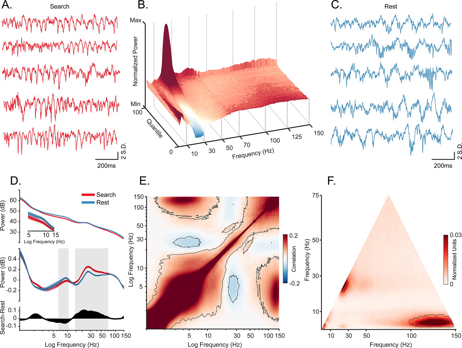
Oscillatory decoupling in CA1 field potentials.
(A) Example traces of broadband local field potential (LFP) in CA1 during search. Data segments were taken from epochs with characteristic high 20–30 Hz power, shown in B (traces were linearly detrended for visualization). (B) Spectral density sorted by 20–30 Hz power. Surface plot shows data segments sorted into quantiles according to 20–30 Hz power, revealing an apparent increase in 5–10 Hz power when 20–30 Hz power is weakest. See Methods for details. (C) Example traces of wideband LFP in CA1 during the rest epoch showing characteristic interactions between <10 Hz and >60 Hz oscillations. Conventions as in A. (D) Top. Mean power spectral density during search (red), and rest (blue). Inset: mean power for low frequencies of main plot, with shaded 95% bootstrap confidence interval (N=42 sessions). Middle. Power spectral density after fitting and subtracting the aperiodic 1/f component during search and rest, with shaded 95% bootstrap confidence intervals. Gray areas show significant differences in power across behavioral epochs (p<0.05, Wilcoxon signed rank test, FDR corrected) Bottom. Power difference between search and rest. (E) Average cross-frequency power comodulogram (N=42 sessions). Dark outline represents areas that were significant in at least 80% of samples (p<0.05, cluster-based permutation test corrected for multiple comparisons). (F) Average bicoherence of the CA1 LFP (N=42 sessions). The dark outline represents areas that were significant in at least 80% of sessions (p<0.05, Monte Carlo test corrected for multiple comparisons). The decoupling is preserved when applying analysis methods sensitive to transient oscillations (Figure 1—figure supplement 2), and when analyzing CA1 LFPs from an additional monkey who moved freely in a search task, and during night-time rest (Figure 1—figure supplement 3).
Figure 1—figure supplement 1
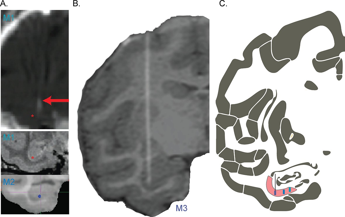
Electrode localization.
(A) Coronal MR and CT images of hippocampal electrode trajectories. CT image of implanted electrode bundle (top) shows the electrode tracts (white puff, red arrow) with deepest electrodes targeting CA1, confirmed in post-explant MR and via functional localization to the pyramidal layer (middle, M1). Red asterisk shown laterally displaced at the depth of probe tip, for visibility. Bottom shows the location of the electrode tip from the CT image placed in a coronal plane of the coregistered MR image for M2. (B) Coronal view of CT-MR coregistered image showing the location of the electrode for M3. (C) Schematic coronal slice showing the location of the CA1 subfield in the hippocampus (pink) with M1, M2, and M3 probe locations from right to left, collapsing across the coronal slab for visualization. Features were adapted from Saleem and Logothetis, 2012 available here. All electrodes used in this study were chronically implanted and individually micro-adjusted in depth to the pyramidal layer.
Figure 1—figure supplement 2
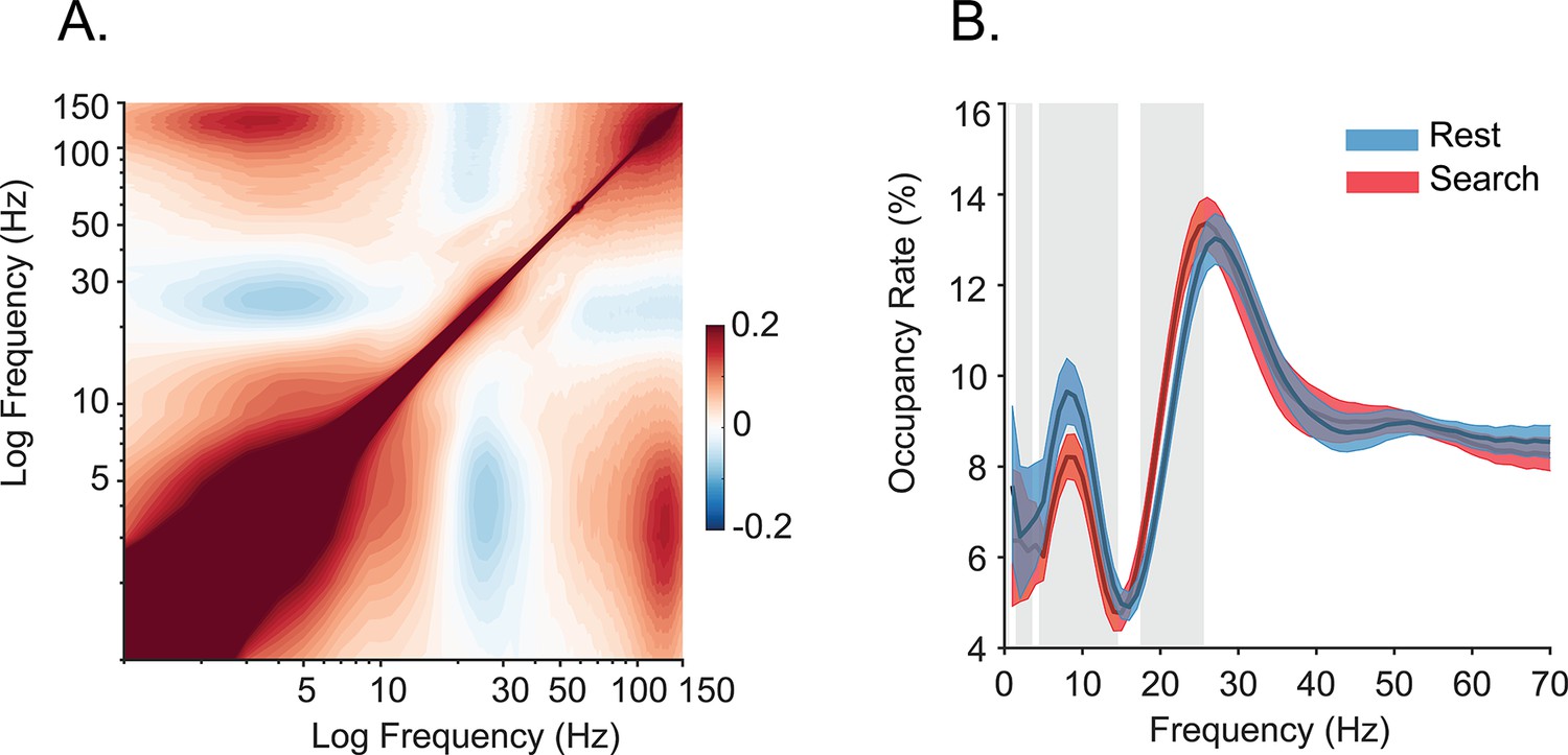
Spectral strength and coupling using alternate analysis methods.
(A) Cross-frequency pairwise correlation of Hilbert (amplitude) envelope (N=42 sessions), which is sensitive to finer temporal coupling resolution than that of the methods used in the main Figure 1. The spectral correlation structure is preserved even at finer temporal resolution. (B) Prevalence of frequency-specific bouts during search (red) and rest (blue) with shaded 95% bootstrap confidence intervals (N=42 sessions, p<0.05, Wilcoxon signed rank test, FDR corrected). Occupancy rate is the percent time spent in a detected bout of the specified frequency (also called ‘Pepisode’).
Figure 1—figure supplement 3
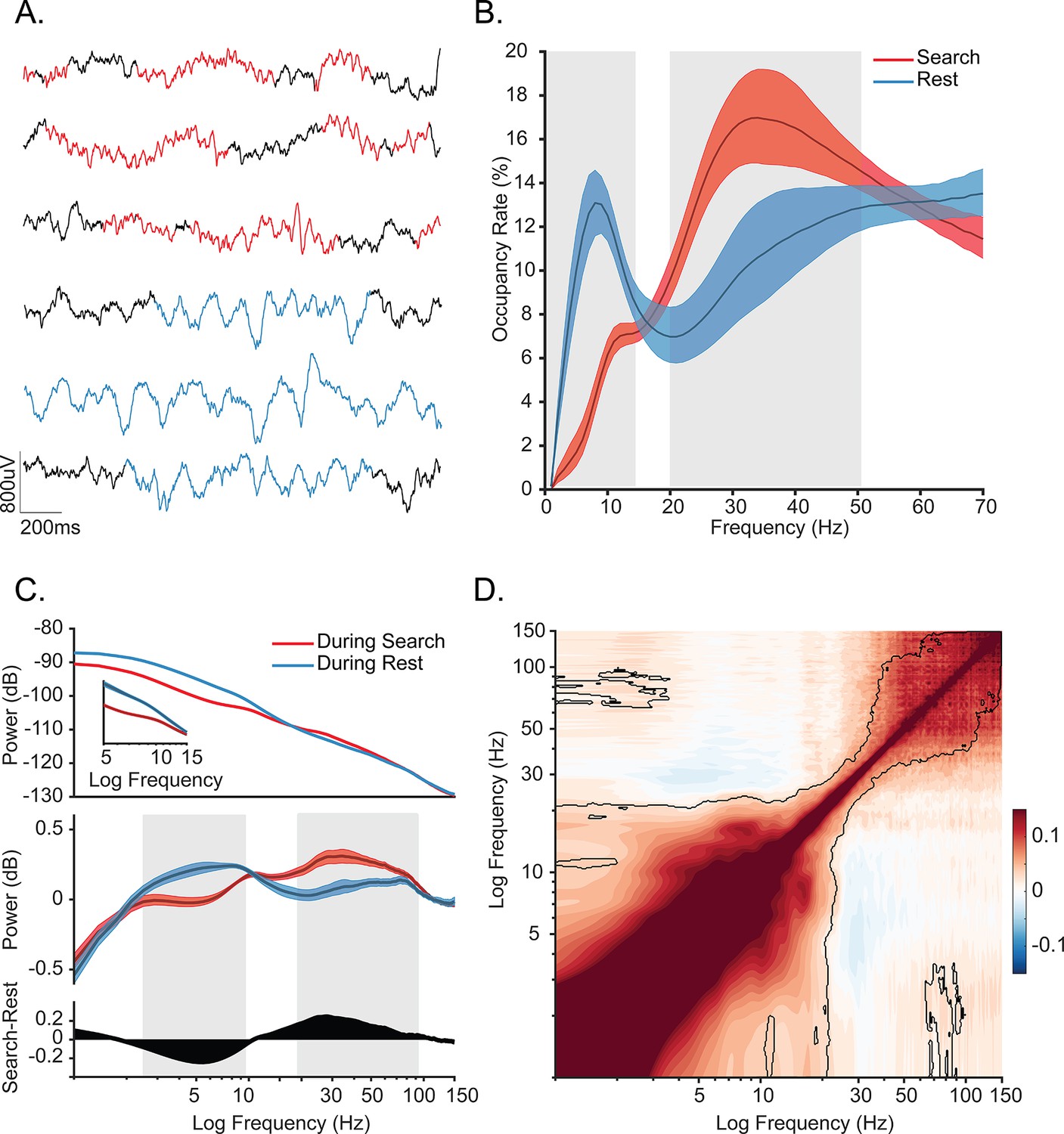
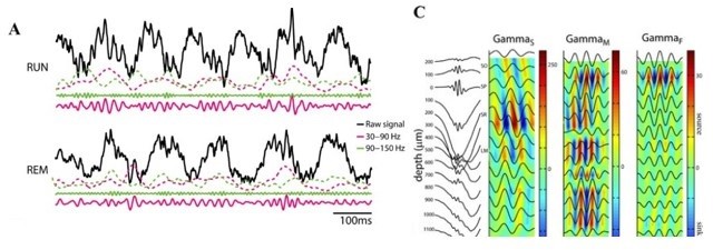
Oscillatory decoupling in CA1 of freely behaving monkeys.
(A) Example detected oscillations in 4–8 Hz and 25–40 Hz frequency bands during awake, free behavior (red), and sleep (blue) shown on the wideband local field potential (LFP) in CA1. (B) Prevalence of frequency-specific bouts during search (red), and rest (blue) with shaded 95% bootstrap confidence intervals (N=18 sessions, p<0.05, Wilcoxon signed rank test, FDR corrected). (C) Top. Mean power spectral density during search (red) and rest (blue). Inset: mean power for low frequencies of the main plot, with shaded 95% bootstrap confidence interval (N=18 sessions). Middle. Power spectral density after fitting and subtracting the aperiodic 1/f component during search and rest, with shaded 95% bootstrap confidence intervals. Gray areas show significant differences in power across behavioral epochs (p<0.05, Wilcoxon signed rank test, FDR corrected) Bottom. Power difference between search and rest. (D) Average cross-frequency power comodulogram (N=18 sessions). Dark outline represents areas that were significant in at least 80% of samples (p<0.05, cluster-based permutation test corrected for multiple comparisons).
Figure 1—figure supplement 4
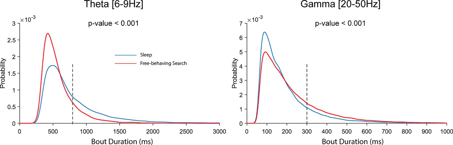
Relative probability distribution of bout durations.
Left. Distribution of detected bout durations for theta (6–9 Hz) oscillation. Red and blue show distribution for detected bouts during active search and offline behavioral states respectively (p<0.05, Wilcoxon signed rank test). For reference, the black dotted line indicates 800 ms, which reflects ~3–6 cycles at 4–8 Hz and is more than twice the duration of the slow sharp-wave ripple (SWR) components (see Figure 2—figure supplement 1). Right. Same as the left plots but for gamma oscillations (20–50 Hz). The black dotted line indicates 300 ms, indicating durations that would exceed two typical 8 Hz cycles. The lower end of the duration distribution is bounded by the duration threshold in the BOSC algorithm.
Figure 2 with 2 supplements
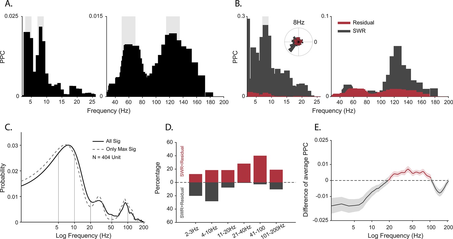
Spike-field coherence and its influence by sharp-wave ripples (SWRs).
(A) Spike-local field potential (LFP) pairwise phase consistency (PPC) spectra for an example unit. Shaded gray shows significant values (p<0.05, permutation test and Rayleigh test, p<0.05). (B) Spike-LFP coherence for spikes during detected SWRs (dark gray) and for spikes remaining after extracting the SWR epochs (‘residual’, red). Light gray shading shows significant difference at p<0.05 in FDR-corrected permutation test for the SWR group. Inset: Normalized histogram of the phase values at 8 Hz, obtained from the spike-LFP coherence analysis shown in A. (C) Probability distribution of observing significant PPC values across all frequencies (solid black line), and only for preferred frequency (frequency with maximum PPC value) before adjusting for SWRs (N=404 units). (D) Difference in the proportion of cells with greater spike-LFP coherence for SWR (gray) and SWR-removed residual (red), for six frequency bands (N=185 units). (E) SWR residual difference of mean spike-LFP coherence. Shading shows 95% bootstrapped confidence interval (N = 185). Positive values indicating greater PPC for residual than SWR groups are shown in red, negative values (SWR>residual) in dark gray.
Figure 2—figure supplement 1
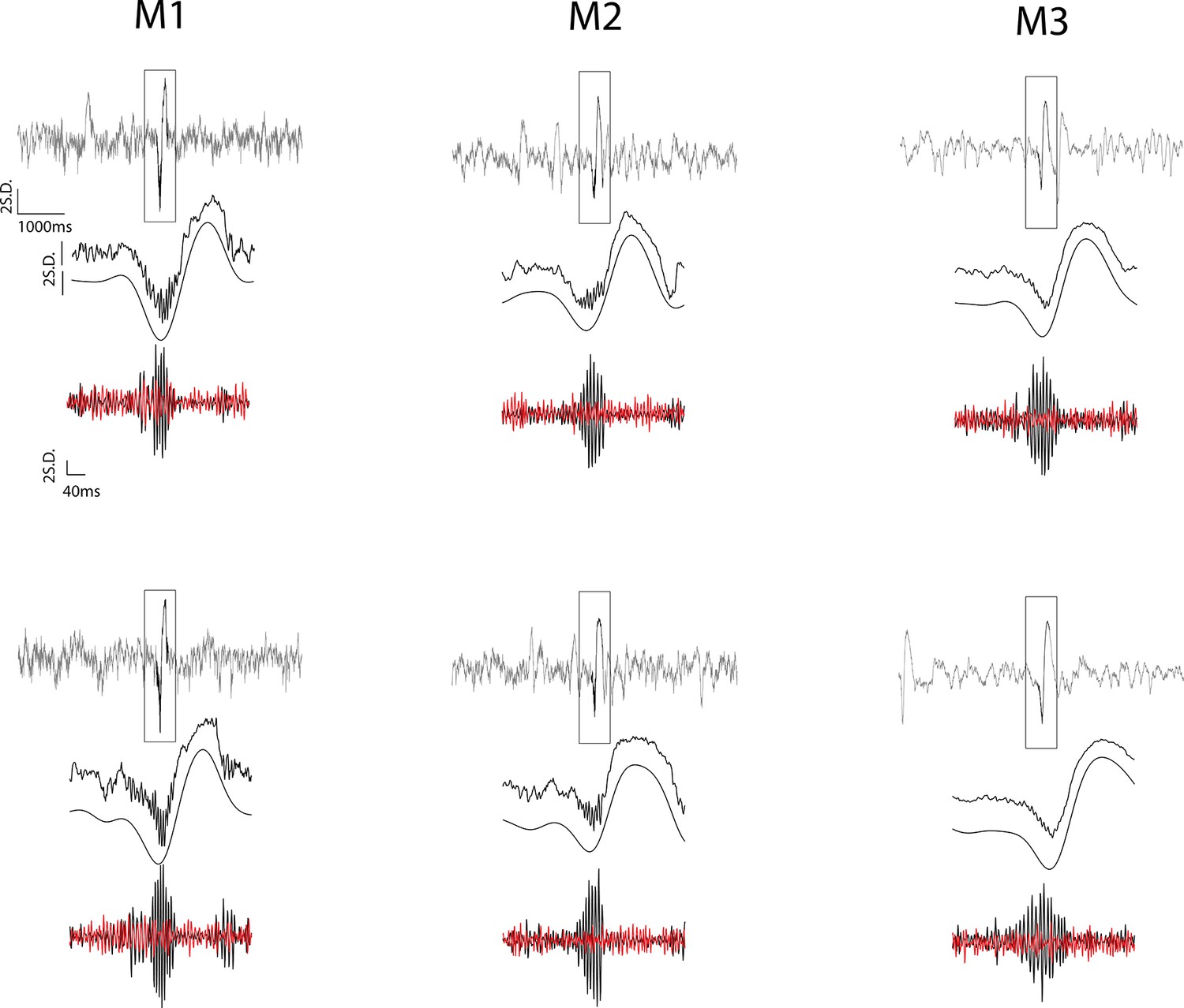
Examples of detected ripple events.
For each example, the first row shows 6 s of z-normalized broadband signal centered at the ripple peak. The second row illustrates the zoomed-in (400 ms) broadband local field potential (LFP) locked to the ripple peak and the narrow-band (<10 Hz) filtered signal. Note that the large amplitude deflection accompanying ripples contains aperiodic spectral energy in the theta band. The third row shows a bandpass (100–250 Hz) filtered trace of the ripple (black) and of a simultaneously recorded signal from a hippocampal channel outside the layer (red), revealing the spatial localization of the ripples. The distant channels were used during ripple detection, to selectively remove high-frequency noise that shares the ripple frequency band, but that are apparent across channels due to volume conduction.
Figure 2—figure supplement 2
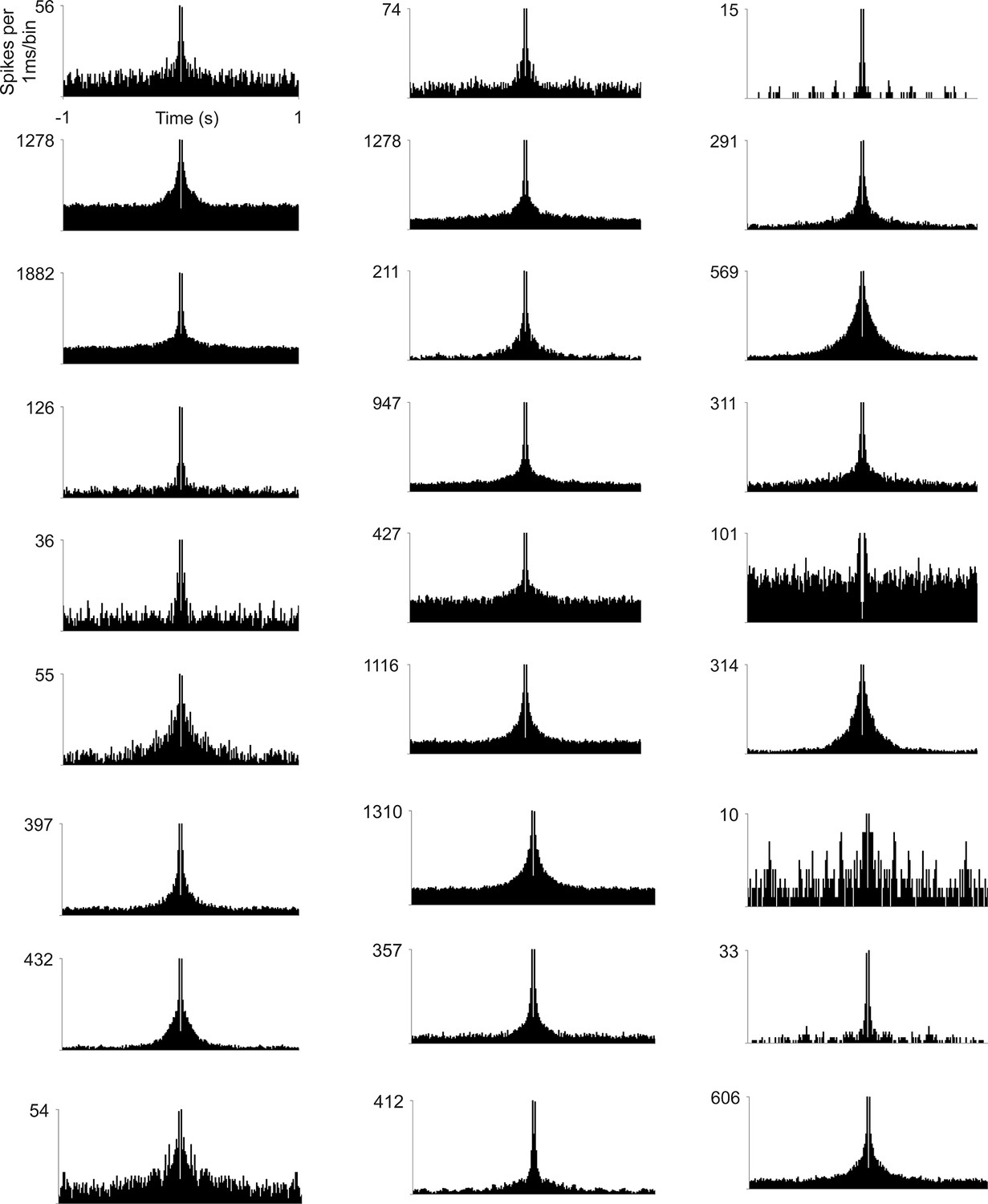
Spike-train autocorrelograms of example hippocampal cells.
Examples were selected to represent different baseline firing rates. Note the absence of any clear temporal modulation in the theta range, including for higher firing rate cells that are predicted to show the strongest modulation. Bin size = 1 ms.
Figure 3
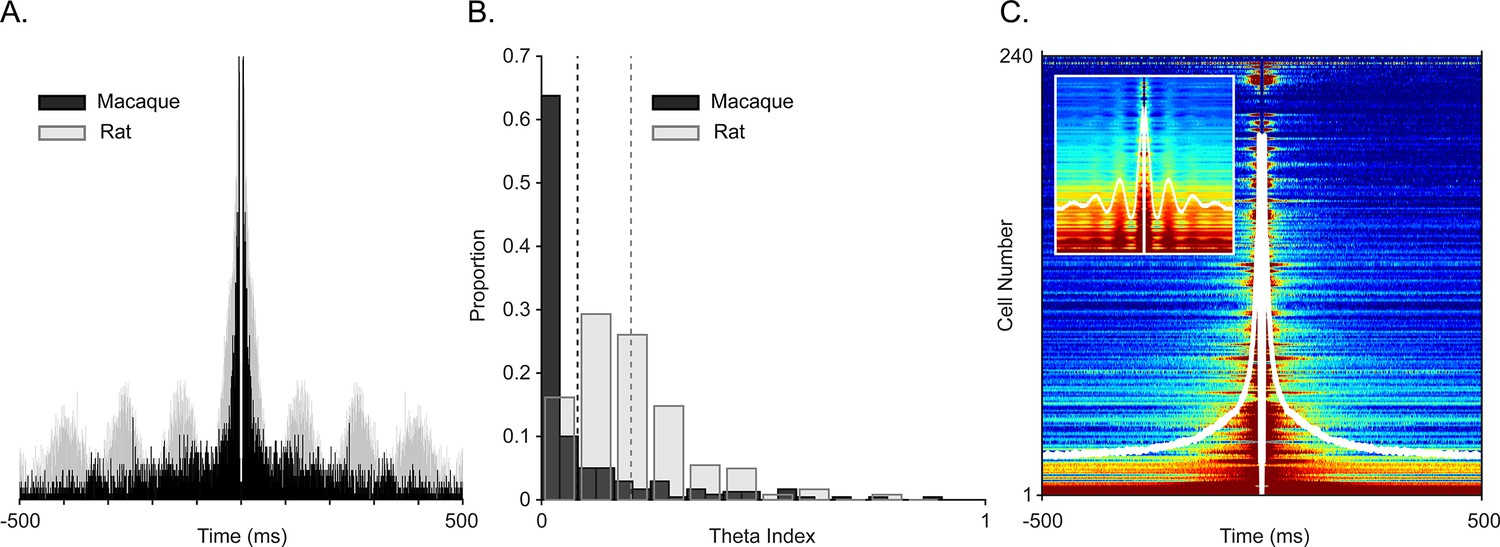
Examining spiking periodicity for theta modulation in macaque hippocampus.
(A) Autocorrelogram of an example ‘theta’ unit from Figure 2A (black, N=945 total spikes) and a theta-modulated unit in rat (gray, N=5655 total spikes). (B) Distribution of the theta index in CA1 units from this study (black, N=240 units), and CA1 units of rat (gray, N=197 units). Dashed lines show mean values, color coded by species. (C) Sorted autocorrelograms of CA1 units, with mean, population ACG shown as a white trace. Inset: same as the main plot but for rats.
Figure 4
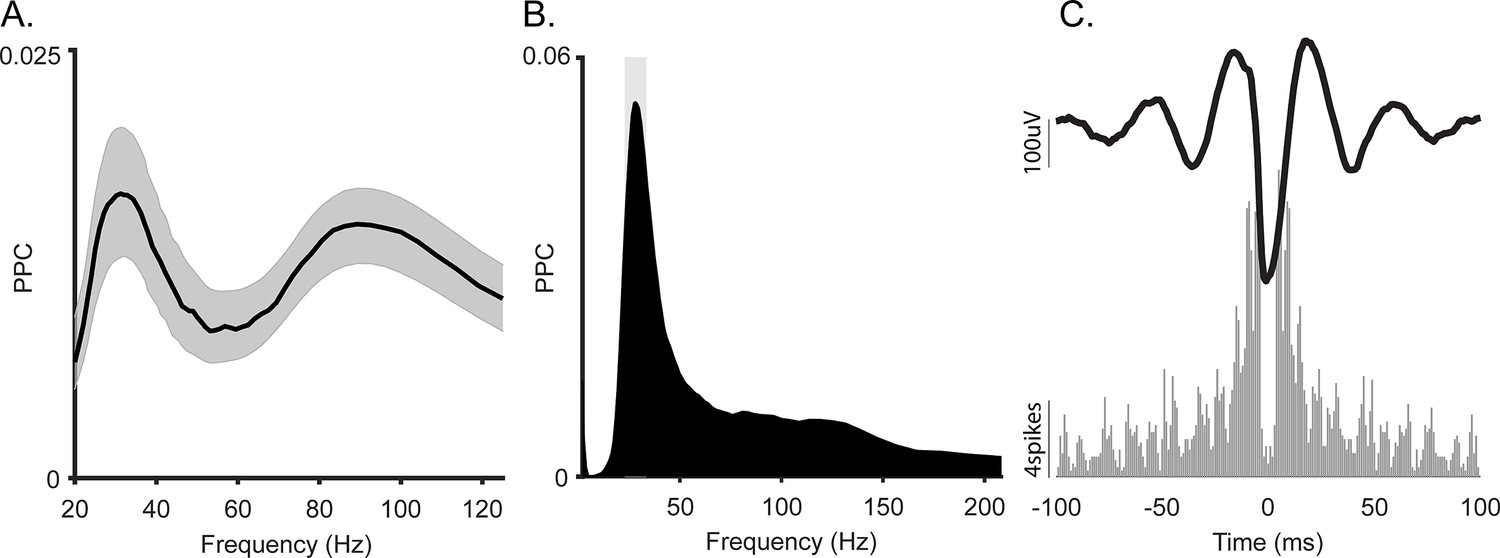
Spike-local field potential (LFP) coherence of the slow gamma oscillation in macaque hippocampus.
(A) Average spike-LFP coherence in gamma frequency range. Shading shows 95% bootstrap confidence interval (N = 404). (B) Spike-LFP coherence for a representative gamma-locked unit. This unit had a significant peak at 30 Hz (p<0.05, permutation test and Rayleigh test, p<0.05). (C) Top: Spike-triggered average LFP of the unit in B. Bottom: Autocorrelogram of the same unit.
Author response image 1
Videos
Video 1
Oscillatory dynamics in monkey CA1 during sleep and waking states.
(Top) Broadband local field potential (LFP) during sleep (blue), and free movement in an enclosure during a search task (red), the 4–8 Hz bandpass filtered LFP, and the 25–50 Hz LFP, shown top to bottom, respectively. Detected bouts in each frequency band are highlighted with blue (sleep) and red (waking). The black vertical line shows 3 SD above the mean. (Bottom) Left: Movement, expressed as the vector norm of angular velocity. The gray horizontal line shows the threshold for movement. Middle: The envelope peak of detected theta (4–8 Hz) bouts plotted as a function of the gamma (25–50 Hz) peaks. Right: 1/f corrected (fitted residual) power spectrum. The distribution of power shifts to higher frequencies during awake compared to sleep.
Additional files
Download links
A two-part list of links to download the article, or parts of the article, in various formats.
Downloads (link to download the article as PDF)
Open citations (links to open the citations from this article in various online reference manager services)
Cite this article (links to download the citations from this article in formats compatible with various reference manager tools)
Theta- and gamma-band oscillatory uncoupling in the macaque hippocampus
eLife 12:e86548.
https://doi.org/10.7554/eLife.86548


