Figures and data in A reservoir of timescales emerges in recurrent circuits with heterogeneous neural assemblies

Figures
Tables
Additional files

13 figures, 1 table and 1 additional file

Figures

Figure 1

Download asset Open asset

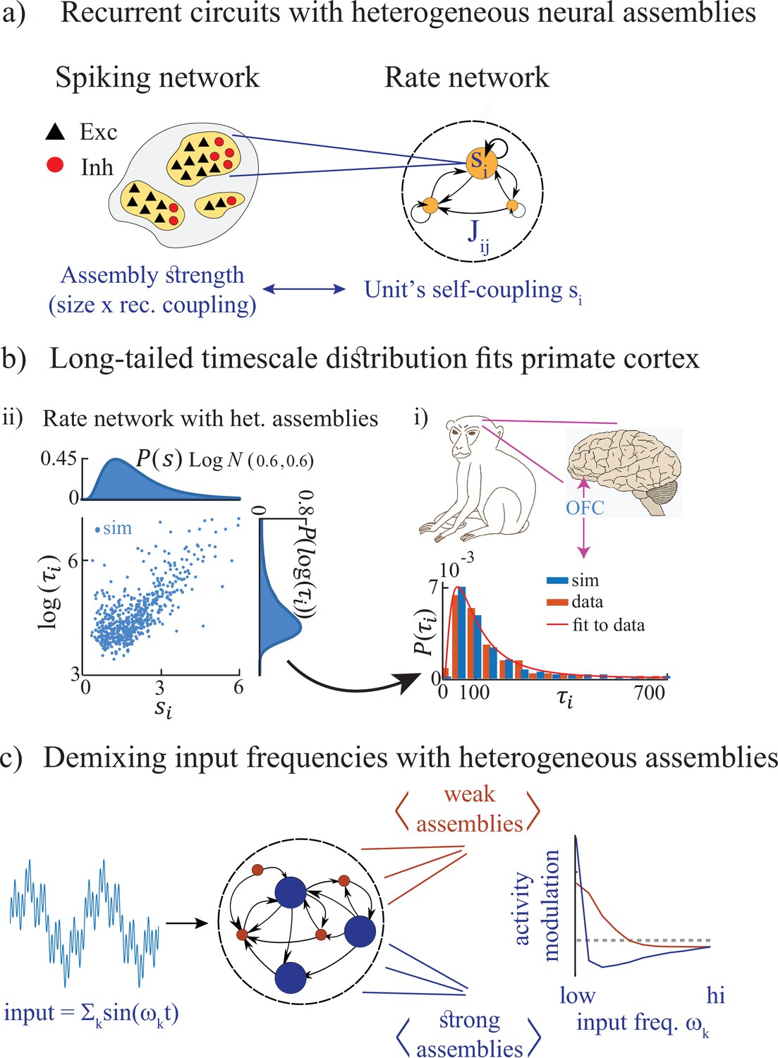
Summary of the main results.

(a) Left: Microscopic model based on a recurrent network of spiking neurons with excitatory and inhibitory cell types, arranged in neural assemblies of heterogeneous sizes. Right: Phenomenological model based on a recurrent network of rate units. Each unit corresponds to an E/I neural assembly, whose size is represented by the unit’s self-couplings $s_{i}$ . (b) A lognormal distribution of self-couplings (representing assemblies of different sizes) generates time-varying activity whose heterogeneous distribution of timescale fits population activity recorded from awake monkey orbitofrontal cortex (data from Cavanagh et al., 2016). (c) When driving our heterogeneous network with broadband time-varying input, comprising a superposition of sine waves of different frequencies, large and small assemblies preferentially entrain with low and high spectral components of the input, respectively, thus demixing frequencies into responses of different populations.

Figure 2

Download asset Open asset

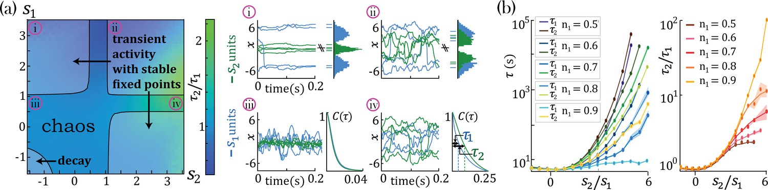
Dynamical and fixed point properties of networks with two self-couplings.

(a) Ratio of autocorrelation timescales $τ_{2} / τ_{1}$ of units with self-couplings $s_{2}$ and $s_{1}$ , respectively ( $τ_{i}$ is estimated as the half width at half max of a unit’s autocorrelation function, see panels iii, iv), in a network with $n_{1} = n_{2} = 0.5$ and $g = 2$ and varying $s_{1}, s_{2}$ . A central chaotic phase separates four different stable fixed point regions with or without transient activity. Black curves represent the transition from chaotic to stable fixed point regimes, which can be found by solving consistently Equation 15, Equation 16, and Equation 18 (using equal to 1 in the latter), see Methods ('Fixed points and transition to chaos' and 'Stability conditions') for details. (i, ii) Activity across time during the initial transient epoch (left) and distributions of unit values at their stable fixed points (right), for networks with $N = 1000$ and (i) $s_{1} = 3.2, s_{2} = - 1.5$ , (ii) $s_{1} = 3.2, s_{2} = 1.2$ . (**iii**, iv) Activity across time (left) and normalized autocorrelation functions $C (τ) / C (0)$ , (right) of units with (iii) $s_{1} = 0.8, s_{2} = - 1.5$ , (iv) $s_{1} = 0.8, s_{2} = 3.2$ . (b) Timescales $τ_{2}, τ_{1}$ (left) and their ratio $τ_{2} / τ_{1}$ (right) for fixed $s_{1} = 1$ and varying $s_{2}$ , as a function of the relative size of the two populations $n_{1} = N_{1} / N, n_{2} = N_{2} / N$ (at $g = 2$ , $N = 2000$ ; average over 20 network realizations). All points in b. were verified to be within the chaotic region using Equation 18.

Figure 3

Download asset Open asset

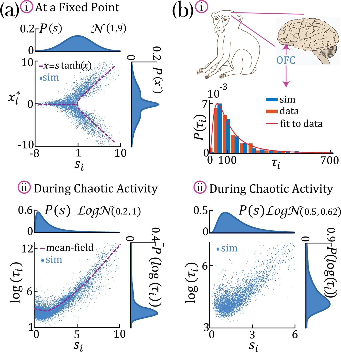
Continuous distributions of self-couplings.

(**a–i**) In a network with a Gaussian distribution of self-couplings (mean $μ = 1$ and variance $σ^{2} = 9$ ), and $g = 2.5$ , the stable fixed point regime exhibits a distribution of fixed point values interpolating between around the zero fixed point (for units with $s_{i} \leq 1$ ) and the multi-modal case (for units with $s_{i} > 1$ ). The purple curve represents solutions to $x = s \tanh (x)$ . (**a,b–ii**) A network with a lognormal distribution of self-couplings (parameters for (a,b) $μ = 0.2, 0.5$ and $σ^{2} = 1, 0.62$ , and $g = 2.5$ ;autocorrelation timescales $τ_{i}$ in units of ms) in the chaotic phase, span several orders of magnitude as functions of the units’ self-couplings $s_{i}$ . (a-ii) Mean-field predictions for the autocorrelation functions and their timescales (purple curve) were generated from Equation 13 and Equation 14 via an iterative procedure, see Methods: 'Dynamic mean-field theory with multiple self-couplings' *, 'An iterative solution'*. (b) Populations of neurons recorded from orbitofrontal cortex of awake monkeys exhibit a lognormal distribution of intrinsic timescales (data from Cavanagh et al., 2016) (panel **b-i**, red), consistent with neural activity generated by a rate network with a lognormal distribution of self-couplings (panel **b-i**, blue; panel **b-ii**). ; We note that Cavanagh et al., 2016 use fitted exponential decay time constants of the autocorrelation functions as neurons’ timescales, while we use the half widths at half max of the autocorrelation functions as the timescales. To bridge these two definitions, we multiplied (Cavanagh et al., 2016) data by a factor of ln(2) before comparing it with our model and presenting it in this figure. The model membrane time constant was assumed to be 3 ms in this example.

Figure 4 with 1 supplement

Download asset Open asset

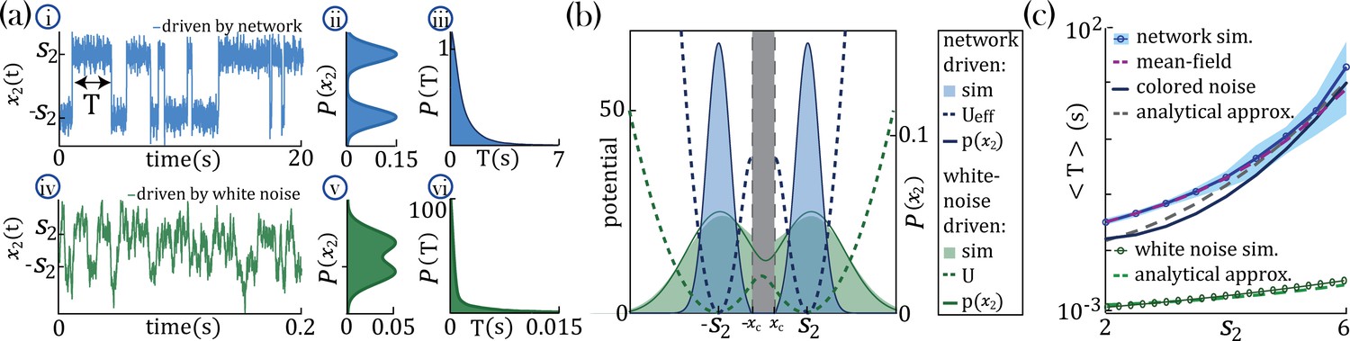
Separation of timescales and metastable regime.

(a) Examples of bistable activity. (**i, iv,i**) - time courses; (**ii, v**) - histograms of unit’s value across time; (**iii, vi**) - histograms of dwell times. (**a–i, ii, iii**) An example of a probe unit $x_{2}$ with $s_{2} = 5$ , embedded in a neural network with $N = 1000$ units, $N_{1} = N - 1$ units with $s_{1} = 1$ and $g = 1.5$ . (**a–iv, v, vi**) An example of a probe unit driven by white noise. Note the differences in the x-axis scalings of the timecourses (**a–i** vs. **a–iv** and **a–iii** vs. **a–vi**).(b) The unified colored noise approximation stationary probability distribution (dark blue curve, Equation 19, its support excludes the shaded gray area) from the effective potential $U_{e f f}$ (dashed blue curve) captures well the activity histogram (light blue area; same as (**a–ii**)); whereas the white noise distribution (dark green curve, obtained from the naive potential $U$ , dashed green curve) captures the probe unit’s activity (light green area; same as (**a–v**)) when driven by white noise, and deviates significantly from the activity distribution when the probe is embedded in our network. (c) Average dwell times, $⟨ T ⟩$ , in the bistable states. Simulation results, mean, and 95%CI (blue curve and light blue background, respectively; An example of the full distribution of the dwell times is given in (**a-iii**)). Mean-field predictions (purple curve) were generated by calculating the average dwell times from a trace of $x_{2}$ , which was produced by solving the mean-field equations; Equation 2 simultaneously and consistently with Equation 3 with $n_{1} = 1$ and $n_{2} = 0$ . The mean first passage time from the unified colored noise approximation (Equation 22, black curve), and for a simplified estimate thereof (Equation 4, gray dashed line) capture well $⟨ T ⟩$ . When driven by white noise (green curve and light green curve are simulation results and simplified estimate using Equation 4, respectively), the probe’s average dwell times are orders of magnitude shorter than with colored noise, exhibiting substantial support of the probe distribution in the region where the crossing between wells happens (allowing frequent crossing,(**a-iv**) green line at $x = 0$ ) and, equivalently, the low value of the potential around its maxima ((b) green dashed line at $x = 0$ ). Comparison of white and colored noise demonstrates the central role of the self-consistent colored noise to achieve long dwell times.

Figure 4—figure supplement 1

Download asset Open asset

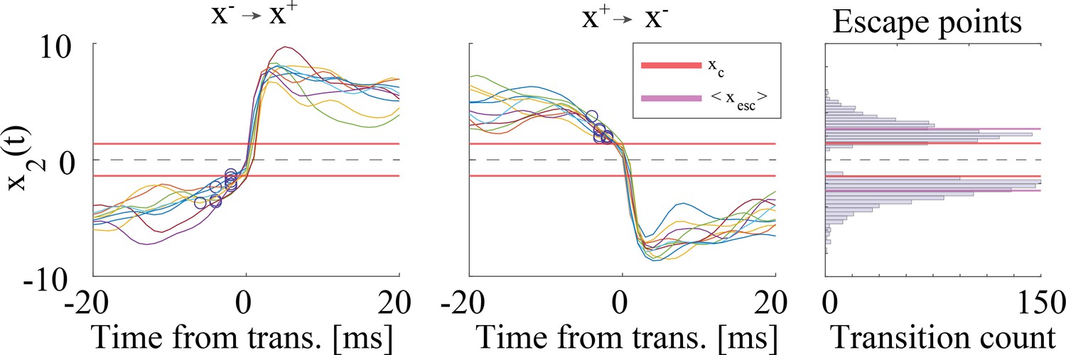
Validation of universal colored noise approximation (UCNA) approach to estimate escape times.

’Escape points’ from one metastable state to the next were estimated from simulations as follows: for a transition from the $x^{-} = - s_{2}$ well towards the $x^{+} = x_{2}$ well (Left panel; analogous calculation for transitions $x^{+} \to x^{-}$ , Center panel), the escape point $x_{e s c}$ was defined as the point where the trajectory starts accelerating towards the target well (positive second derivative). The distribution of escape points (Right panel) predominantly lied outside of the forbidden region (93.8% of escape points had $| x_{e s c} | > x_{c}$ ). Parameters: same as in Figure 4a–i, $s_{2} = 5$ . See Methods ('Universal colored-noise approximation to the Fokker-Planck theory') for further details.

Figure 5

Download asset Open asset

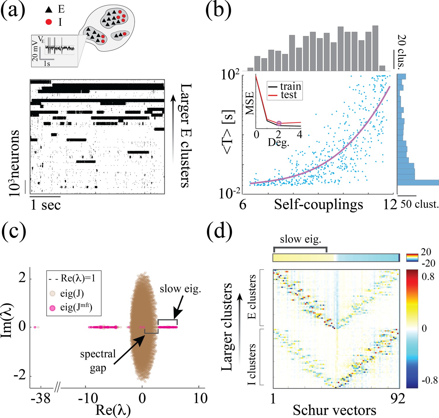
*Heterogeneity of timescales in E-I spiking networks*.

(a) Top: Schematic of a spiking network with excitatory (black) and inhibitory populations (red) arranged in assemblies with heterogeneous distribution of sizes. Bottom: In a representative trial, neural assemblies activate and deactivate at random times generating metastable activity (one representative E neuron per assembly; larger assemblies on top; representative network of $N = 10, 000$ neurons), where larger assemblies tend to activate for longer intervals. (b) The average activation times <T> of individual assemblies (blue dots; the average was calculated across 100s simulation and across all neurons within the same assembly for all assemblies in 20 different network realizations; self-coupling units are in [mV], see Methods section). Fit of $\log (T) = a_{2} s_{E}^{2} + a_{1} s_{E} + a_{0}$ with $a_{2} = 0.14, a_{1} = 1.97, a_{0} = 5.51$ (pink curve). Inset: cross-validated model selection for polynomial fit. As the assembly strength (i.e. the product of its size and average recurrent coupling) increases, <T> increases, leading to a large distribution of timescales ranging from 20 ms to 100s. (c) Eigenvalue distribution of the full weight matrix $J$ (brown) and the mean-field-reduced weight matrix $J^{M F}$ (pink). (d) The Schur eigenvectors of the weight matrix $J^{M F}$ show that the slow (gapped) Schur eigenvalues (top) are associated with eigenvectors corresponding to E/I cluster pairs (bottom). See Appendix (e) Spiking network model for more details and for the scaling to larger networks.

Figure 6

Download asset Open asset

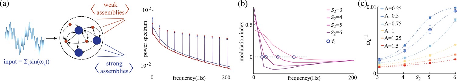
Network response to broadband input.

(a) Power spectrum density of a network driven by time-dependent input comprising a superposition of 11 sinusoidal frequencies (see main text for details). Maroon and navy curves represent average power spectrum density in $s_{1}$ and $s_{2}$ populations, respectively; circles indicate the peak in the power spectrum density amplitudes at each frequency; amplitude A = 0.5, $g = 3.0$ , $s_{1} = 1$ , and $s_{2} = 4$ . (b) Modulation index of the power spectrum density amplitudes as a function of frequency in networks with $s_{1} = 1$ and various $s_{2}$ . The blue circles mark the cutoff frequency $f_{c}$ where the modulation index changes sign. (c) Cutoff period, $2 π ω_{c}^{- 1}$ , as a function of self-coupling $s_{2}$ for different input amplitudes. An inversely proportional relation between the cutoff period and the amplitude of the broadband signal is present.

Appendix 1—figure 1

Download asset Open asset

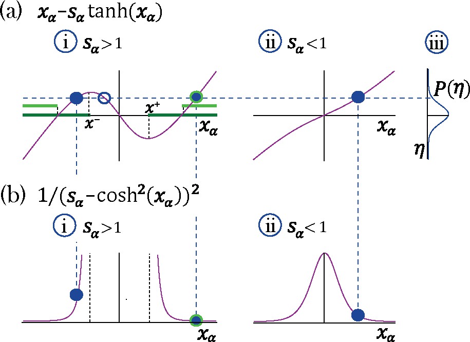
Transition to chaos with multiple self-couplings: Fixed point solutions and stability.

(**a–i**) The fixed point curve $x_{α} - s_{α} \tanh x_{α}$ , from Equation 15, for $s_{α} > 1$ . Stable solutions are allowed within the dark green region. (**b–i**) The shape of a unit’s contribution to stability $q^{- 1} = (s_{α} - \cosh {x_{α}}^{2})^{- 2}$ , from Equation 18. Stable solutions of $x_{α} - s_{α} \tanh x_{α} = η$ , filled blue circles in (**a–i**), with different $| x |$ values contribute differently to stability. At the edge of chaos only a fixed point configuration with all units contributing most to stability (minimal $q^{- 1}$ ) is stable, light green region in (**a–i**).(**a–ii**) The curve $x_{α} - s_{α} \tanh x_{α}$ for $s_{α} < 1$ . (**a-iii**) A possible distribution of the Gaussian mean-field $η$ . A representative fixed point solution is illustrated by the dashed blue line: for $s_{α} < 1$ a single solution exists for all values of $η$ , (filled blue circle in a-ii); For $s_{α} > 1$ multiple solutions exist (**a–i**) for some values of $η$ ; some of them lead to instability (empty blue circle in a-i). The other two solutions may lead to stability (filled blue circles in a-ii), although only one of them will remain stable at the edge of chaos (encircled with green line in a-i).

Appendix 1—figure 2

Download asset Open asset

Network dynamics with identical self-couplings, adopted from Stern et al., 2014.

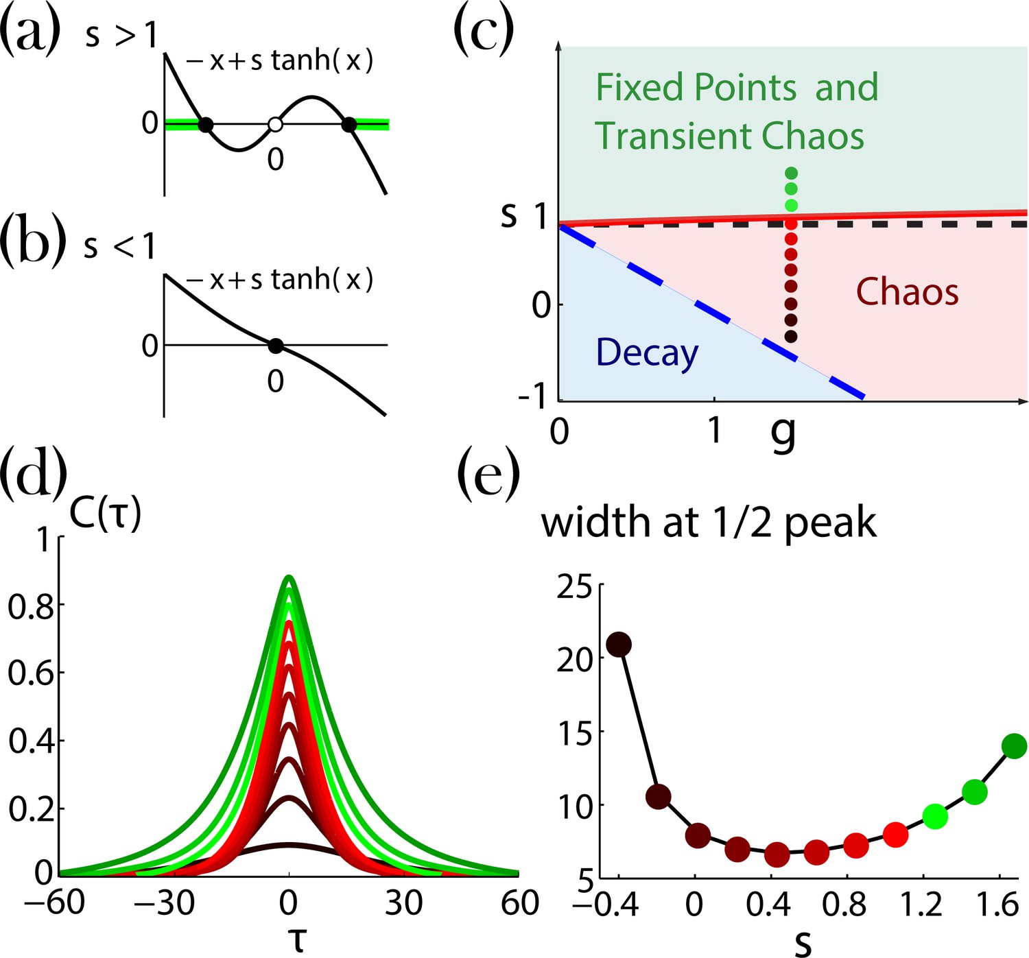
(**a,b**) Graphical solutions to Equation 29. (a) For $s > 1$ there are two stable non-zero solutions (full black circles) and an unstable solution at zero (open black circle). The green background over the $x$ axis denotes the regions of allowed activity values at the stable fixed point on the transition line to chaos (solid red curve in (c)).(b) For $s < 1$ there is a single stable solution (full black circle) at zero. (c) Regions of the network dynamics over a range of $s$ and $g$ values. Below the long dashed blue line, any initial activity in the network decays to zero. Above the solid red curve, the network exhibits transient irregular activity that eventually settles into one out of a number of possible nonzero stable fixed points. In the region between these two curves, the network activity is chaotic. Colored circles denote, according to their locations on the phase diagram and with respect to their colors, the values of $s$ (ranging from 1.6 and decreasing with steps of 0.2) and $g = 1.5$ , used for the autocorrelation functions $C (τ)$ in (d; corrected version of Figure 4a in Stern et al., 2014). (e) Widths at half peak (values of $τ$ ’s in the main text notation) of the autocorrelation functions in (d).

Appendix 2—figure 1

Download asset Open asset

Synaptic weight matrices of clustered spiking networks.

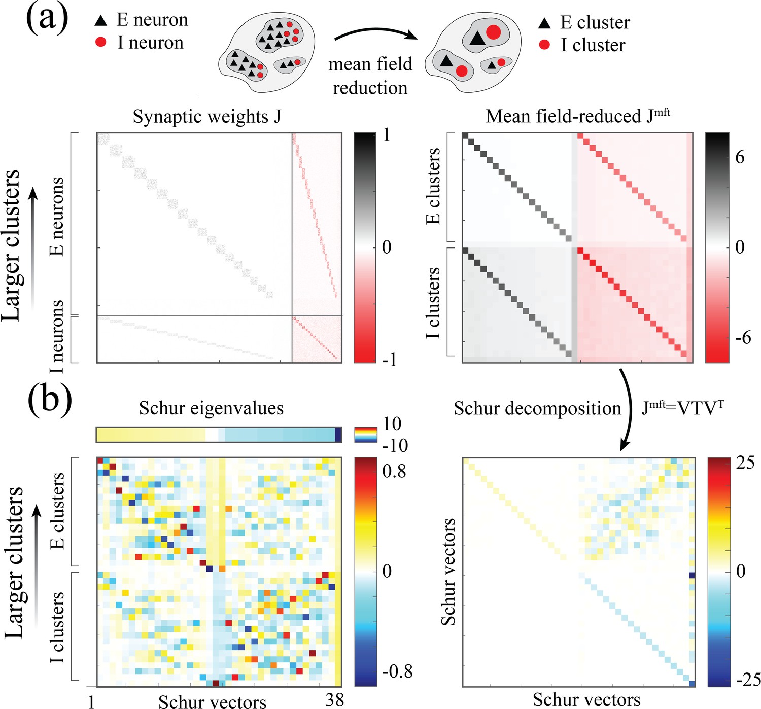
Synaptic weight matrices of a clustered spiking networks. (a) Left: Synaptic weight matrix $J$ of a clustered spiking network with $N = 2000$ neurons, exhibiting the E/I four submatrices, where diagonal blocks within each submatrix reveal the E/I clustered structure (larger to smaller clusters, top to bottom in each submatrix). Right: $2 (p + 1)$ -dimensional mean-field-reduced synaptic weight matrix $J^{M F}$ corresponding to the full matrix on the left. Populations are ordered as follows: $p + 1$ excitatory clusters (larger to smaller, top to bottom), background excitatory population, $p + 1$ inhibitory clusters, background inhibitory population. For each pair of populations, the value in $J^{M F}$ is obtained from the corresponding block in $J$ by summing its column values (presynaptic inputs) and averaging over the rows (postsynaptic neurons belonging to the population). (b) Right: Schur decomposition of $J^{M F} = V T V^{T}$ into an upper triangular matrix $T$ . Left: Schur eigenvectors (columns of $V$ , bottom) sorted from larger to smaller Schur eigenvalue (top). Larger Schur eigenvalues are associated with eigenvectors whose loadings are on larger E/I cluster pairs.

Appendix 2—figure 2

Download asset Open asset

Metastable attractor dynamics in clustered spiking networks.

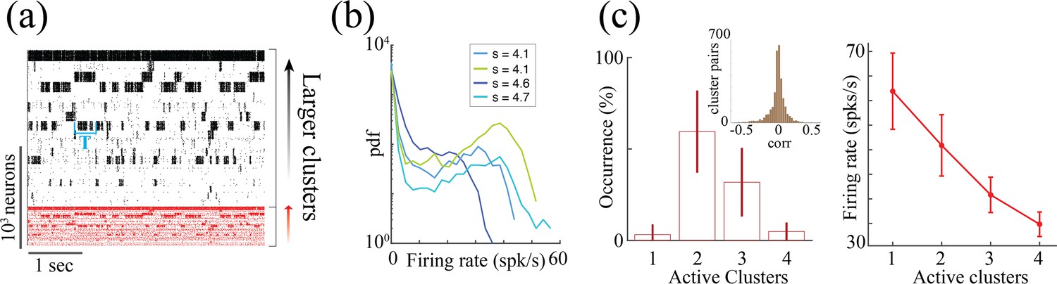
Metastable attractor dynamics in clustered spiking networks. (a) Metastable activity from all clustered neurons in a representative trial of a network with $N = 2000$ neurons (larger to smaller clusters, top to bottom; action potentials from excitatory and inhibitory neurons, black and red, respectively). (b) Firing rate distributions of four representative neurons from the network in (a) exhibit bimodal distributions (colors represent clusters with different self-couplings; spike counts estimated in 100ms bins over 20 trials of 200 seconds duration). (c) Left: Metastable attractor dynamics unfolds through different network configurations with a range of simultaneously active clusters from one to four (average occurrence of each configuration across 20 networks as fraction of total simulation time). Inset: Metastable dynamics are uncorrelated across clusters (distribution of pairwise Pearson correlations between clusters’ firing rates, 0.01±0.12, mean±SD; 20 networks). Right: The firing rate of neurons in active clusters depend on how many clusters are simultaneously active, with higher firing rates in configurations with less co-active clusters (mean and SD across 20 networks).

Appendix 2—figure 3

Download asset Open asset

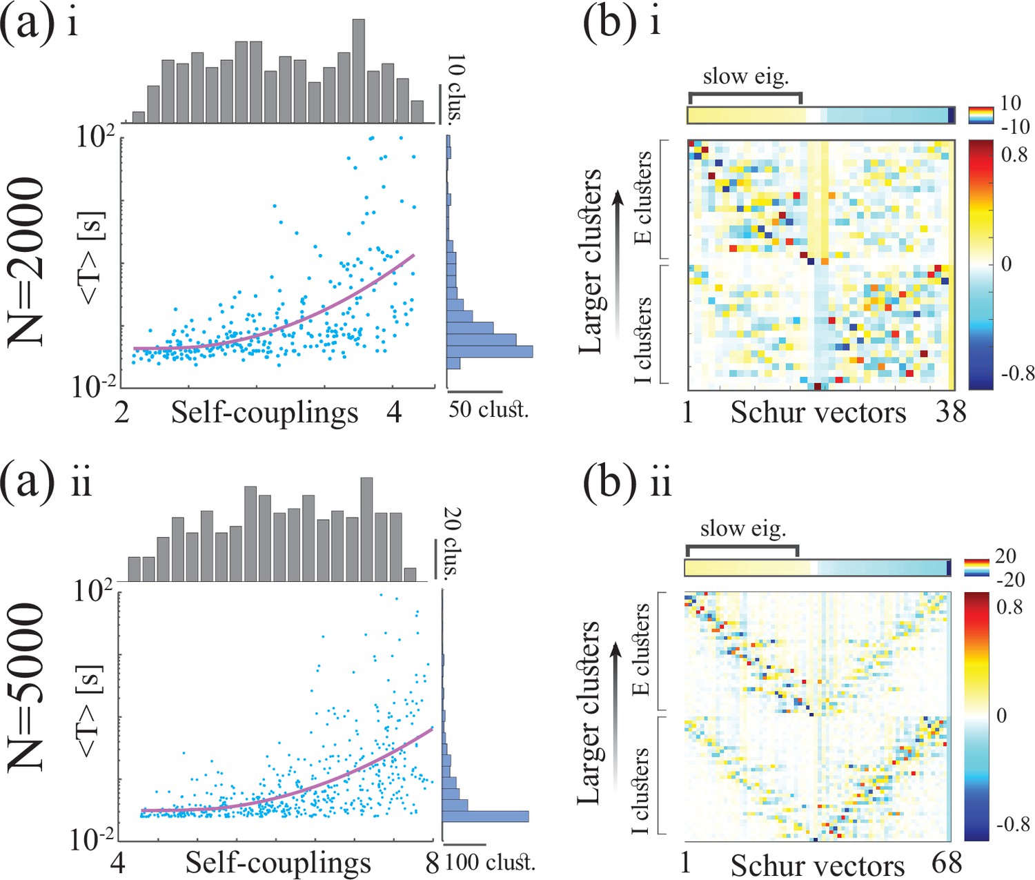
Metastable activity and timescale distribution in networks of $N = 2000, 5000$ neurons (top and bottom rows, respectively).

Panels (a) and (b) have the same notations as Figure 5b, and Figure 5d, respectively. The fits of average activation time $T$ vs. self-coupling $\log (T) = a_{2} s_{E}^{2} + a_{1} s_{E} + a_{0}$ yielded $a_{2} = 0.44, a_{1} = 2.06, a_{0} = 1.04$ for $N = 2000$ ; and $a_{2} = 0.093, a_{1} = - 0.88, a_{0} = 0.45$ for $N = 5000$ .

Appendix 2—figure 4

Download asset Open asset

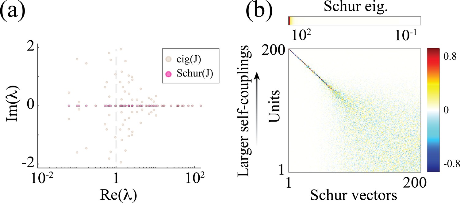
Chaotic rate network of $N = 200$ units (self-couplings drawn from a lognormal distribution with parameters $μ = 0.2, σ = 2$ ).

(a) Eigenvalue distribution (brown) and Schur eigenvalues (pink) of the synaptic weight matrix $J$ . (b) The Schur eigenvectors of $J$ corresponding to large positive Schur eigenvalues have loadings localized on units with larger self-couplings, with a similar structure to the Schur eigenvectors in the spiking networks in Appendix 2-figure 3 .

Appendix 3—figure 1

Download asset Open asset

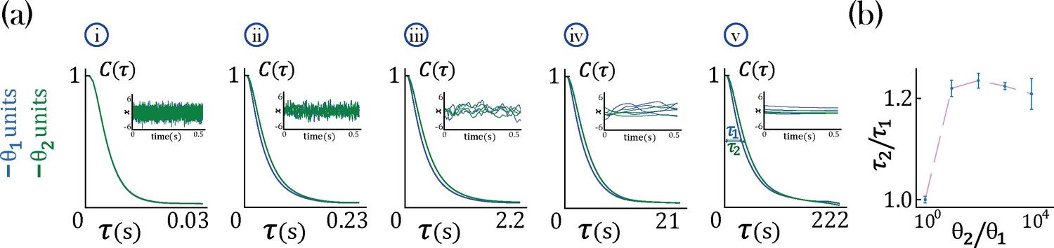
Timescale analysis for an RNN with two-time constants $θ_{i}$ , Equation 31, governing equal populations of neurons ( $N_{1} = N_{2} = 1000$ ) and gain $g = 2.5$ .

(a) Average autocorrelation function for each population. The insert shows the dynamics of individual neurons from each population: blue for neurons with timeconstant $θ_{1}$ and green for neurons with timeconstant $θ_{2}$ . In the networks considered here, $θ_{1} = 0.1$ ms is kept constant while: $θ_{2} = 0.1$ ms (i), $θ_{2} = 1.0$ ms (ii), $θ_{2} = 10.0$ ms (iii), $θ_{2} = 100.0$ ms (iv), $θ_{2} = 1000.0$ ms (v). (b) Population timescale ratio $τ_{2} / τ_{1}$ for fixed timeconstant $θ_{1} = 0.1$ ms and varying $θ_{2}$ .

Tables

Table 1

Parameters for the clustered network used in the simulations.

Model parameters for clustered network simulations
Parameter	Description	Value
$J_{E E}$	E-to-E synaptic weights	$0.9 / \sqrt{N}$ [mV]
$J_{I E}$	E-to-I synaptic weights	$0.9 / \sqrt{N}$ [mV]
$J_{E I}$	I-to-E synaptic weights	$2.7 / \sqrt{N}$ [mV]
$J_{I I}$	I-to-I synaptic weights	$5.4 / \sqrt{N}$ [mV]
$J_{E 0}$	E-to-E synaptic weights	$3.7 / \sqrt{N}$ [mV]
$J_{I 0}$	I-to-I synaptic weights	$3.3 / \sqrt{N}$ [mV]
$J_{E E}^{+}$	Potentiated intra-assembly E-to-E weight factor	$14 \sqrt{N / 2000}$
$J_{I I}^{+}$	Potentiated intra-assembly I-to-I weight factor	$5 \sqrt{N / 2000}$
$g_{E I}$	Potentiation parameter for intra-assembly I-to-E weights	$10 \sqrt{N / 2000}$
$g_{I E}$	Potentiation parameter for intra-assembly E-to-I weights	$8 \sqrt{N / 2000}$
$r_{e x t}$	Average baseline afferent rate to E and I neurons	5 [spks/s]
$V_{E}^{t h r}$	E-neuron threshold potential	1.43 [mV]
$V_{I}^{t h r}$	I-neuron threshold potential	0.74 [mV]
$V^{r e s e t}$	E- and I-neuron reset potential	0 [mV]
$τ_{m}$	E- and I-neuron membrane time constant	20 [ms]
$τ_{r e f r}$	E- and I-neuron absolute refractory period	5 [ms]
$τ_{s}$	E- and I-neuron synaptic time constant	5 [ms]

Additional files

MDAR checklist: https://cdn.elifesciences.org/articles/86552/elife-86552-mdarchecklist1-v2.docx
Download elife-86552-mdarchecklist1-v2.docx

Download links

A two-part list of links to download the article, or parts of the article, in various formats.

Downloads (link to download the article as PDF)

Open citations (links to open the citations from this article in various online reference manager services)

Mendeley

Cite this article (links to download the citations from this article in formats compatible with various reference manager tools)

Merav Stern
Nicolae Istrate
Luca Mazzucato

(2023)

A reservoir of timescales emerges in recurrent circuits with heterogeneous neural assemblies

eLife 12:e86552.

https://doi.org/10.7554/eLife.86552

Figures

Summary of the main results.

Dynamical and fixed point properties of networks with two self-couplings.

Continuous distributions of self-couplings.

Separation of timescales and metastable regime.

Validation of universal colored noise approximation (UCNA) approach to estimate escape times.

Heterogeneity of timescales in E-I spiking networks.

Network response to broadband input.

Transition to chaos with multiple self-couplings: Fixed point solutions and stability.

Network dynamics with identical self-couplings, adopted from Stern et al., 2014.

Synaptic weight matrices of clustered spiking networks.

Metastable attractor dynamics in clustered spiking networks.

Metastable activity and timescale distribution in networks of $N = 2000, 5000$ neurons (top and bottom rows, respectively).

Chaotic rate network of $N = 200$ units (self-couplings drawn from a lognormal distribution with parameters $μ = 0.2, σ = 2$ ).

Timescale analysis for an RNN with two-time constants $θ_{i}$ , Equation 31, governing equal populations of neurons ( $N_{1} = N_{2} = 1000$ ) and gain $g = 2.5$ .

Tables

Parameters for the clustered network used in the simulations.

Additional files

MDAR checklist

Download links

Downloads (link to download the article as PDF)

Open citations (links to open the citations from this article in various online reference manager services)

Cite this article (links to download the citations from this article in formats compatible with various reference manager tools)

Be the first to read new articles from eLife

Share this article

Cite this article

Summary of the main results.

Dynamical and fixed point properties of networks with two self-couplings.

Continuous distributions of self-couplings.

Separation of timescales and metastable regime.

Validation of universal colored noise approximation (UCNA) approach to estimate escape times.

Heterogeneity of timescales in E-I spiking networks.

Network response to broadband input.

Transition to chaos with multiple self-couplings: Fixed point solutions and stability.

Network dynamics with identical self-couplings, adopted from Stern et al., 2014.

Synaptic weight matrices of clustered spiking networks.

Metastable attractor dynamics in clustered spiking networks.

Metastable activity and timescale distribution in networks of N=2000,5000 neurons (top and bottom rows, respectively).

Chaotic rate network of N=200 units (self-couplings drawn from a lognormal distribution with parameters μ=0.2,σ=2).

Timescale analysis for an RNN with two-time constants θi, Equation 31, governing equal populations of neurons (N1=N2=1000) and gain g=2.5.

Parameters for the clustered network used in the simulations.

MDAR checklist

Downloads (link to download the article as PDF)

Open citations (links to open the citations from this article in various online reference manager services)

Cite this article (links to download the citations from this article in formats compatible with various reference manager tools)

Metastable activity and timescale distribution in networks of $N = 2000, 5000$ neurons (top and bottom rows, respectively).

Chaotic rate network of $N = 200$ units (self-couplings drawn from a lognormal distribution with parameters $μ = 0.2, σ = 2$ ).

Timescale analysis for an RNN with two-time constants $θ_{i}$ , Equation 31, governing equal populations of neurons ( $N_{1} = N_{2} = 1000$ ) and gain $g = 2.5$ .