Evidence for adolescent length growth spurts in bonobos and other primates highlights the importance of scaling laws
- Domestication Lab, Konrad Lorenz Institute of Ethology, Department of Interdisciplinary Life Sciences, University of Veterinary Medicine Vienna, Austria
- Behavioral Ecology and Ecophysiology, Department of Biology, University of Antwerp, Belgium
- Centre for Research and Conservation, Royal Zoological Society of Antwerp, Belgium
- SALTO Agro- and Biotechnology, Odisee University of Applied Sciences, Belgium
- Max Planck Institute for Evolutionary Anthropology, Germany
- Max-Planck-Institute of Animal Behaviour, Germany
- Comparative BioCognition, Institute of Cognitive Science, University of Osnabrück, Germany
- Endocrinology Laboratory, German Primate Center, Leibniz Institute for Primate Research, Germany
- Leibniz ScienceCampus Primate Cognition, German Primate Center, Leibniz Institute for Primate Research, Germany
Figures
Figure 1 with 1 supplement
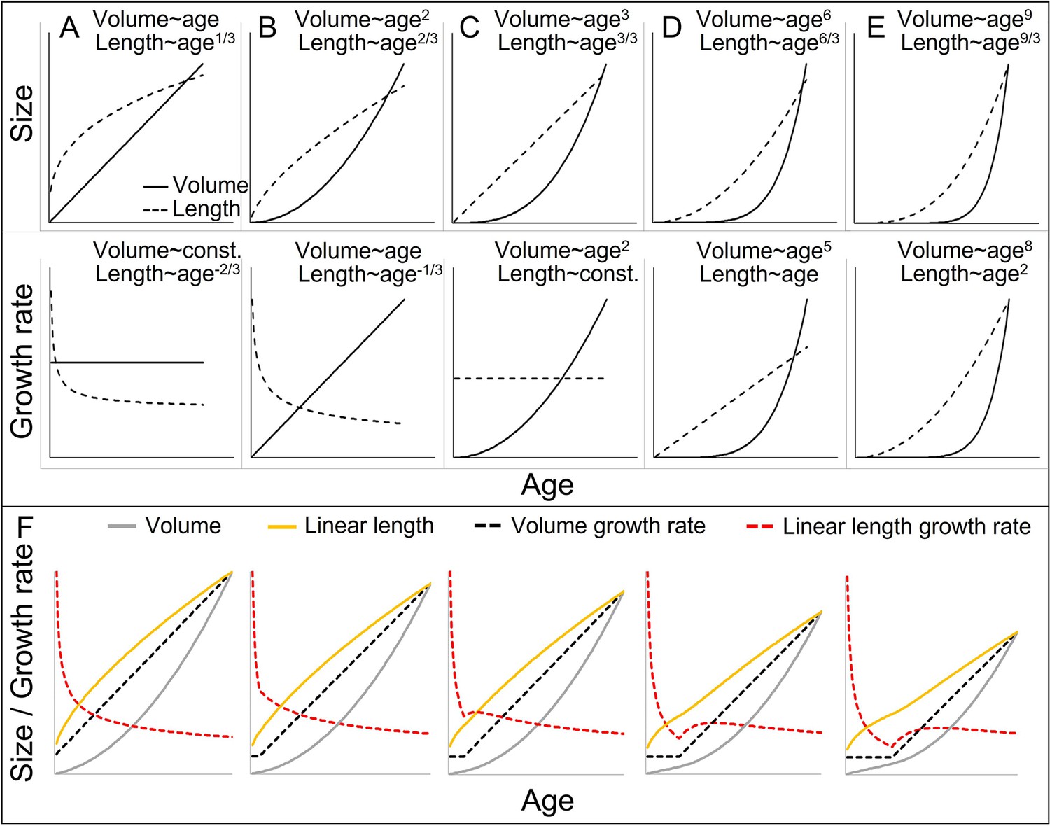
Cubic isometric relationship between volume (~weight) and length growth, and likelihood to detect an existing growth spurt (GS) in linear length (schematic).
(A–E) Top/bottom: Absolute size and growth rate (=1st derivation of size). From left to right: Increasingly fast acceleration of volume (~weight) growth and the aligned length growth, from (A) no acceleration (constant volume growth rate and linear increase in volume) through (B) constant acceleration (linear increase in volume growth rate and quadratic increase in volume) to (C) quadratic acceleration of volume growth rate (cubic increase in volume), and (D, E) even faster volume growth acceleration. Due to the cubic relationship, these volume growth rates would align with decreasing (A, B) or constant length growth rates (C), whereas a detectable acceleration in length growth rate may only be found in cases of very fast acceleration in volume growth rate (D, E). Therefore, the current dichotomy between absent and detectable length GSs would only differentiate between (A–C) and (D, E). Another consequence is that, in non-aquatic animals, a cubic relationship is more likely in smaller animals, whereas in larger animals like humans or bonobos, the relationship tends to follow a lower power of 2.5 or even 2 only, as a result from limitation on the bearable weight of a skeletal construction which relates to the sectional area of bones (for more details see e.g., Juul et al., 1995). This means that in case of an equal volume growth acceleration, an aligned acceleration in linear length growth may become more likely detectable in larger animals simply because of the different underlying scaling laws. (F) The above scaling rules lead to further dynamics depending on the temporal overlap of the curves, making length GSs more pronounced and detectable with increasing size (from left to right). A GS in linear length is detectable if the acceleration resulting from the volume-GS exceeds the deceleration in length growth rate that results from the cubic relationship, with the last one becoming weaker with increasing size, respective age. The figure shows how a change from a constant to a linearly accelerating volume growth rate (like in A and B; equal levels of acceleration) results in different levels of acceleration in linear length growth rate depending on the age/size at which this change occurs, from left (change right after birth, only deceleration in length growth rate) (equal to B) to right (change at late age, strong acceleration in length growth rate). Additionally, this figure highlights that even if both volume and linear length show a GS and are perfectly aligned, the linear length growth rate reaches its peak and starts declining again at a time when volume growth rate still increases. See also Figure 1—figure supplement 1 for non-linear acceleration in volume growth rate.
Figure 1—figure supplement 1
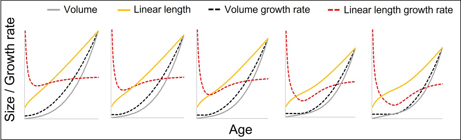
The figure shows how a change from a constant to a quadratically accelerating volume growth rate at a certain body size (identical levels of acceleration) results in different levels of acceleration in linear length growth rate depending on the age (in fact, body size) at which this change occurs, from left (change right after birth at small body size, only slight acceleration in linear length growth rate) to right (change at late age and larger body size, strong acceleration in length growth rate).
Figure 2 with 2 supplements
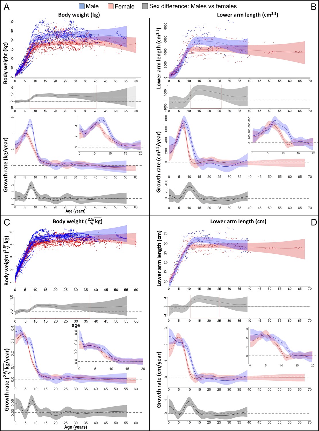
Growth trajectories in body weight and forearm length, and the importance of comparing them at the relevant dimension.
Fitted values and 95% CIs from Generalized Additive Mixed Models (GAMMs) are shown, implementing variability in trajectories across individuals and zoos. (A, B) Investigating both weight and length growth at the dimension of weight growth reveals pronounced growth spurts (GSs) in both which are strongly aligned with each other in timing and amplitude (see also Figure 4A for easier comparison). (C, D) If instead examined at the scale of one-dimensional length growth, weight, and length growth curves still align with each other but the GSs are not so easily detectable anymore. However, the GS is still evident in female growth, but appears at a younger age than if scale corrected (A, B). The potential fast decrease in growth rate after birth was not covered by linear length data (first half year of age: 2 arm and 854 [729 male] weight measures).
Figure 2—figure supplement 1
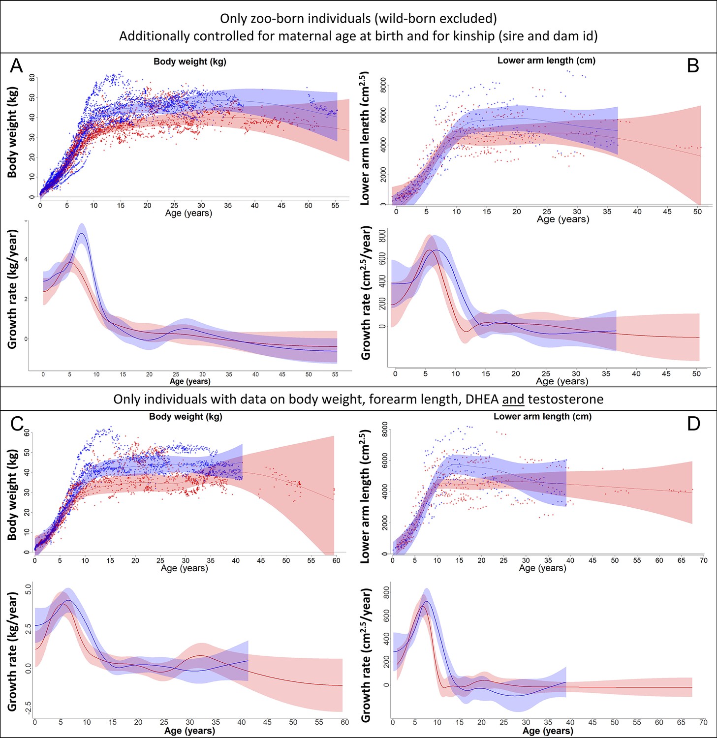
Our results on body weight (left) and forearm length (right) remained the same if (A, B) only zoo-born individuals were considered (which also allowed to additionally control for kinship [dam and sire] and maternal age at birth) or if (C, D) only those individuals were considered for which data on body weight, forearm length, dehydroepiandrosterone (DHEA), and testosterone were available.
Blue = males; red = females. 95% confidence intervals are plotted.
Figure 2—figure supplement 2
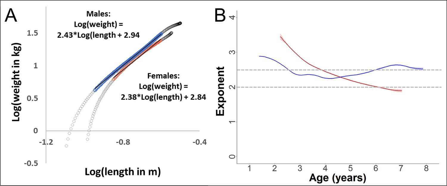
Validation of the scaling relationship between forearm length and body weight during growth in our study.
Since weight and length were not measured pairwise, we used the fitted values from the respective Generalized Additive Mixed Models (GAMMs). The power-exponent of the relationship is calculated as the linear slope of the log–log plot. (A) Log–log plot of weight over length, with data from the growth period (range 0–10 years of age in females and 0–14 years in males, grey circles). During the period of a linear relationship (coloured, blue = males and red = females), the slope (and thus the exponent of the relationship between the non-transformed variables) was 2.4 for both sexes. (B) For the same data used for slope calculation in (A), but with dynamic slope calculation using the first derivative of the GAM-smooth. The exponent for males was relatively stable around 2.5 during this age period, whereas the value decreased in females, reaching about 2.0 towards the end of the growth spurt (see results section, Figures 2—4).
Figure 3 with 3 supplements
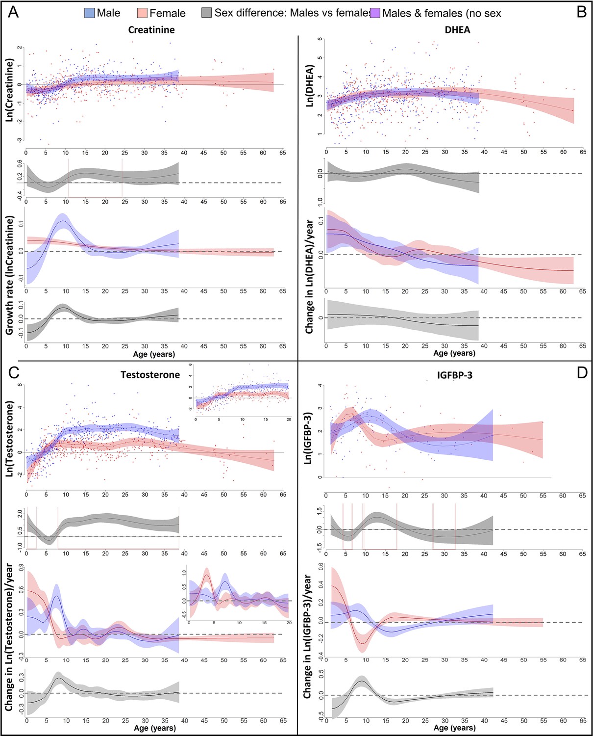
Physiological changes during ontogeny: markers of muscle growth (creatinine), adrenarche (dehydroepiandrosterone, DHEA), and adolescence (testosterone and insulin-like growth factor-binding protein 3 [IGFBP-3]).
Fitted values and 95% CIs from Generalized Additive Mixed Models (GAMMs) are shown, which implement variability in trajectories across individuals and zoos. (A) Males showed a pronounced growth spurt (GS) in lean body respective muscle mass, resulting in larger lean body mass in males compared to females where such a GS was not detectable. Be aware though that corrected creatinine values before the age of 3–4 years may be less reliable (Emery Thompson et al., 2012). (B) DHEA levels increased fastest during the first 5 years of life and reached maximal levels at ~15 years. (C) Testosterone levels increased during development in both sexes, but in males, testosterone levels increased longer and reached higher adult levels. They increased fastest at 3.5–4 years in females and 7 years in males. Testosterone levels decreased again after the age of ~30 years of age. (D) IGFBP-3 levels showed a peak of similar height in males and females, occurring at a younger age in females than males.
Figure 3—figure supplement 1
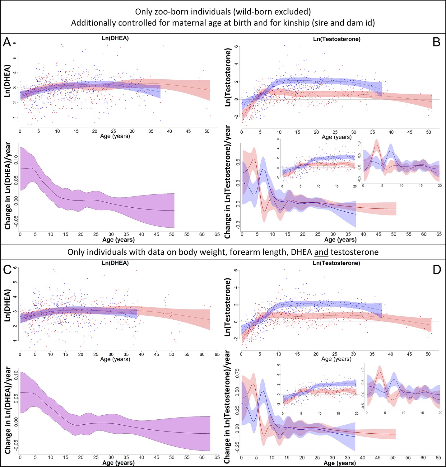
Our results on dehydroepiandrosterone (DHEA) (left) and testosterone (right) remained the same if (A, B) only zoo-born individuals were considered (which also allowed to additionally control for kinship [dam and sire] and maternal age at birth) or if (C, D) only those individuals were considered for which data on body weight, forearm length, DHEA, and testosterone were available.
Blue = males, red = females. 95% confidence intervals are plotted.
Figure 3—figure supplement 2
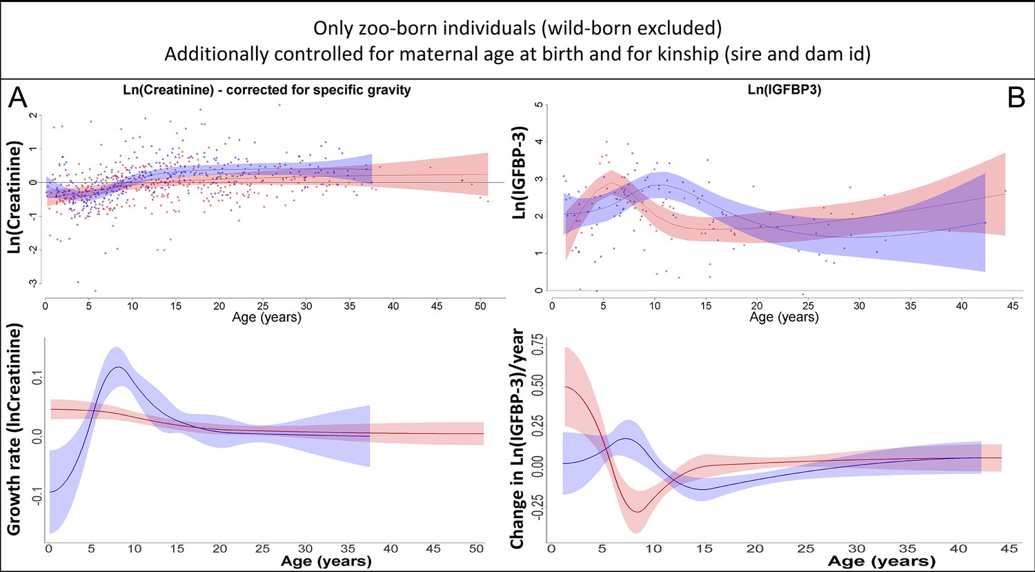
Our results on creatinine (A) and insulin-like growth factor-binding protein 3 (IGFBP-3) (B) remained the same if only zoo-born individuals were considered (which also allowed to additionally control for kinship [dam and sire] and maternal age at birth).
Blue = males, red = females. 95% confidence intervals are plotted.
Figure 3—figure supplement 3
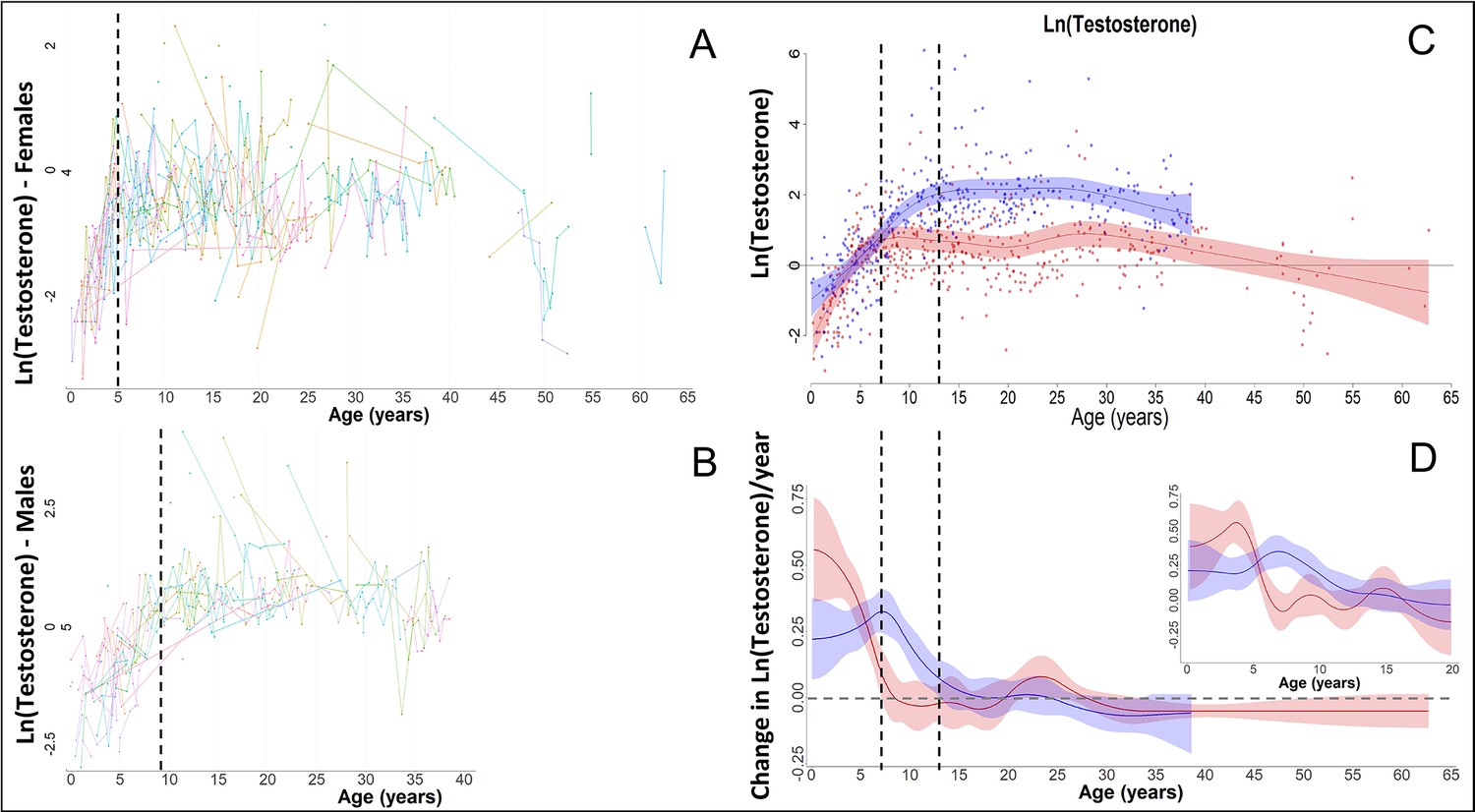
In our raw data, females and males showed a fast increase in testosterone, as also previously shown for bonobos (Behringer et al., 2014), with females (red) reaching maximal levels around the age of 5, and males (blue) around the age of 9 years.
However, this fast change was not appropriately modelled by our Generalized Additive Mixed Models (GAMMs) if the ‘automatic’ estimation of the smoothing parameters was used, leading to strong oversmoothing and much later ages at which maximal levels were attained, and at which the increase in testosterone levels ceased, in both sexes. Therefore, we applied a fixed smoothing parameter to our testosterone GAMMs of sp = 1, which allowed for higher ‘wiggliness’ and thus faster changes, and which solved the issue.
Figure 4
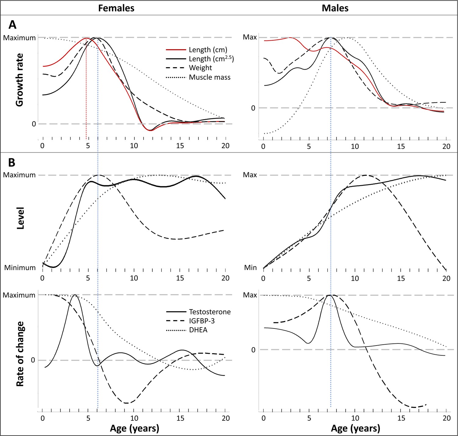
Direct comparison of age trajectories in growth patterns and physiological parameters until the age of 20 years.
All curves are the same as in Figures 2 and 3, and for the respective variability and uncertainty in the trajectories including the occurrence, level, and timing of peaks see the 95% CIs in Figures 2 and 3. Blue and red dotted line: Age at peak growth velocity in cm2.5/year (blue) and in cm/year (red; females only). (A) Change of growth rate over age in weight, forearm length, and lean body respective muscle mass (measured as urinary creatinine). (B) Levels (top) and rate of change (bottom) in urinary testosterone, insulin-like growth factor-binding protein 3 (IGFBP-3) and dehydroepiandrosterone (DHEA) levels.
Tables
Table 1
Statistical results of Generalized Additive Mixed Models (GAMMs) on growth and physiology.
Blue: Interaction term results from a separate model (see methods section). Red: Special model structure for insulin-like growth factor-binding protein 3 (IGFBP-3) models (random intercept per individual, random smooth per zoo not sex specific; for details see methods). §: including maternal primiparity, rearing conditions (hand- vs. mother-reared) and zoo- vs. wild-born (see methods section). *: . Model p-values result from null model comparison. Est. = Estimate.
| Factor variables | Reference Category | Body weight (kg) | Body weight (√kg*) | Lower arm length (cm) | Lower arm length (cm2.5) | ||||||||||||
|---|---|---|---|---|---|---|---|---|---|---|---|---|---|---|---|---|---|
| Est. | SE | t | p | Est. | SE | t | p | Est. | SE | t | p | Est. | SE | t | p | ||
| (Intercept) | 22.4 | 0.10 | 222 | <0.001 | 3.17 | 0.01 | 581 | <0.001 | 25.2 | 0.06 | 443 | <0.001 | 3504 | 19.1 | 183 | <0.001 | |
| Males | Females | 4.10 | 0.13 | 30.8 | <0.001 | 0.20 | 0.01 | 26.9 | <0.001 | 1.26 | 0.19 | 6.77 | <0.001 | 567 | 63.0 | 9.00 | <0.001 |
| Smooth term variables | edf | Ref.df | F | p | edf | Ref.df | F | p | edf | Ref.df | F | p | edf | Ref.df | F | p | |
| Age trajectories | |||||||||||||||||
| Females | 9.12 | 9.39 | 82.3 | <0.001 | 9.00 | 9.19 | 52.1 | <0.001 | 8.32 | 8.71 | 120 | <0.001 | 8.44 | 8.78 | 54.7 | <0.001 | |
| Males | 9.53 | 9.67 | 116 | <0.001 | 9.42 | 9.52 | 52.4 | <0.001 | 7.75 | 8.37 | 115 | <0.001 | 8.06 | 8.56 | 43.2 | <0.001 | |
| Males | Females | 8.53 | 8.84 | 6.36 | <0.001 | 9.04 | 9.26 | 7.42 | <0.001 | 7.05 | 7.77 | 5.34 | <0.001 | 6.71 | 7.48 | 4.49 | <0.001 |
| Random smooths | |||||||||||||||||
| Sampling date per zoo | 103 | 175 | 2.85 | <0.001 | 97.6 | 175 | 2.53 | <0.001 | 10.7 | 44.0 | 0.49 | <0.001 | 7.05 | 37.0 | 0.47 | <0.001 | |
| Age trajectory per individual | 600 | 1544 | 14.4 | <0.001 | 577 | 1545 | 10.5 | <0.001 | 148 | 336 | 14.6 | <0.001 | 151 | 336 | 20.5 | <0.001 | |
| Age trajectory per rearing§ | 2.12 | 53.0 | 0.12 | <0.001 | 27.6 | 53.0 | 2.29 | <0.001 | 0.00 | 48.0 | 0.00 | 0.116 | 0.00 | 48.0 | 0.00 | 0.022 | |
| Female age trajectory per zoo | 32.1 | 175 | 0.29 | <0.001 | 21.9 | 175 | 0.18 | <0.001 | 0.01 | 23.0 | 0.00 | 0.070 | 0.02 | 23.0 | 0.00 | 0.055 | |
| Male age trajectory per zoo | 35.1 | 168 | 0.35 | <0.001 | 61.0 | 168 | 0.91 | <0.001 | 6.69 | 26.0 | 0.88 | <0.001 | 10.9 | 26.0 | 1.45 | <0.001 | |
| R2adj (deviance explained) | 0.995 (99.5%) | 0.997 (99.7%) | 0.988 (99.1%) | 0.986 (99.0%) | |||||||||||||
| N (p-value) | 8355 (<0.001) | 8355 (<0.001) | 641 (<0.001) | 641 (<0.001) | |||||||||||||
| Factor variables | Reference Category | Ln(Creatinine) | Ln(DHEA) | Ln(Testosterone) | Ln(IGFBP-3) | ||||||||||||
| Est. | SE | t | p | Est. | SE | t | p | Est. | SE | t | p | Est. | SE | t | p | ||
| (Intercept) | –0.02 | 0.07 | –0.96 | 0.337 | 2.99 | 0.04 | 84.2 | <0.001 | 0.43 | 0.05 | 9.15 | <0.001 | 2.06 | 0.08 | 25.6 | <0.001 | |
| Males | Females | 0.14 | 0.04 | 3.97 | <0.001 | –0.05 | 0.04 | –1.09 | 0.276 | 0.97 | 0.10 | 9.34 | <0.001 | 0.04 | 0.12 | 0.34 | 0.732 |
| Smooth term variables | edf | Ref.df | F | p | edf | Ref.df | F | p | edf | Ref.df | F | p | edf | Ref.df | F | p | |
| Daytime | 1.00 | 1.00 | 8.98 | 0.003 | 1.77 | 1.94 | 2.04 | 0.116 | 1.00 | 1.00 | 2.46 | 0.118 | 1.00 | 1.00 | 2.94 | 0.089 | |
| Age trajectories | |||||||||||||||||
| Females | 2.64 | 2.99 | 6.17 | <0.001 | 4.69 | 5.44 | 6.16 | <0.001 | 8.48 | 8.85 | 19.2 | <0.001 | 5.04 | 5.65 | 5.39 | <0.001 | |
| Males | 4.45 | 4.77 | 20.4 | <0.001 | 2.97 | 3.38 | 9.77 | <0.001 | 8.33 | 8.81 | 30.6 | <0.001 | 3.98 | 4.66 | 5.53 | <0.001 | |
| Males | Females | 4.41 | 4.73 | 3.73 | 0.016 | 1.00 | 1.00 | 0.24 | 0.622 | 8.05 | 8.63 | 8.24 | <0.001 | 3.24 | 3.62 | 3.27 | 0.010 |
| Random smooths | |||||||||||||||||
| Sampling date per zoo | 24.7 | 56.0 | 2.61 | <0.001 | 33.0 | 55.0 | 10.5 | <0.001 | 25.4 | 58.0 | 3.46 | <0.001 | - | - | - | - | |
| Age trajectory per individual | 42.0 | 385 | 0.18 | <0.001 | 14.88 | 392 | 0.05 | 0.031 | 66.4 | 397 | 0.38 | <0.001 | 0.00 | 103 | 0.00 | 0.819 | |
| Age trajectory per rearing§ | 0.00 | 28.0 | 0.00 | 0.191 | 0.00 | 28.0 | 0.00 | 0.651 | 1.79 | 28.0 | 0.24 | <0.001 | - | - | - | - | |
| Female age trajectory per zoo | 7.55 | 34.0 | 0.57 | <0.001 | 2.77 | 60.0 | 0.06 | 0.042 | 6.66 | 66.0 | 0.26 | <0.001 | 0.00 | 35.0 | 0.00 | 0.554 | |
| Male age trajectory per zoo | 0.00 | 33.0 | 0.00 | 0.087 | 0.58 | 60.0 | 0.01 | 0.13 | 2.46 | 63.0 | 0.05 | 0.006 | - | - | - | - | |
| R2adj (deviance explained) | 0.424 (48.7%) | 0.488 (52.7%) | 0.712 (75.5%) | 0.235 (28.7%) | |||||||||||||
| N (p-value) | 766 (<0.001) | 782 (0.001) | 802 (<0.001) | 163 (0.003) | |||||||||||||
Table 2
Evidence of length growth spurts (GSs) from published literature using linear length growth.
Measures of linear length growth are taken of: Body length or height = B, Crown-rump/Shoulder-rump/Anterior trunk length = CR/SR/AT, Lower/Upper/Full arm length = LA/UA/A, Thigh/Tibia/Leg length = TH/TI/L. Methods: in zoos = direct measurements, in wild populations = photogrammetry, except on Macaca ochreata (direct on trapped animals). Growth rate acceleration can be seen as proof of a GS, but considering scale correction, a GS is also very likely in case of a period with constant linear length growth rate, and would be possible in cases of just a slowdown in deceleration. For markers of adolescence see Appendix 1—table 1. m = male, f = female, w = wild, z = zoo.
| Species (w/z) | Changes in length growth rate | ||||||
|---|---|---|---|---|---|---|---|
| Acceleration | Constant (plateau) | Slowdown in deceleration | No slowdown in deceleration | Aligned with weight-GS | Comments | Publication | |
| Macaca assamensis (w) | m + f (LA) | Not available | Acceleration if scale corrected | Anzà et al., 2022; Berghänel et al., 2015 | |||
| Macaca fuscata (z) | m + f (B), m (AT, UA) | m (TH, L) | m (LA), f (LA) | f (UA) | Yes (little earlier) | Hamada, 1994; Hamada et al., 1999; Hamada and Yamamoto, 2010 | |
| Macaca nemestrina (z) | m + f (AT, CR, A, LA, L) | Yes | Nishikawa, 1985; Tarrant, 1975 | ||||
| Macaca arctoides (z) | m (CR) | Yes | Few individuals | Faucheux et al., 1978 | |||
| Macaca mulatta (z) | (B, TI)1 | m + f (CR) | Yes (little earlier) | 1Unknown sex, few individuals | Tanner et al., 19901; van Wagenen and Catchpole, 1956 | ||
| Macaca ochreata (w) | m + f (CR) | Yes | Schillaci and Stallmann, 2005 | ||||
| Theropithecus gelada (w) | m + f (SR) | Not available | Lu et al., 2016 | ||||
| Papio anubis (z) | m (CRL) | m + f (A) | m (TH), f (CRL, TH) | Yes (little earlier) | Leigh, 2009 | ||
| Papio hamadryas (z) | m (CR) | f (CR) | Yes (m) | Coarse data | Crawford et al., 1997 | ||
| Mandrillus sphinx (z) | m + f (CR) | Yes | Setchell et al., 2001 | ||||
| Pan troglodytes (z) | m + f (B) | Yes | Hamada and Udono, 2002 | ||||
| Pongo pygmaeus (z) | m + f (B, LA) | Yes | Two individuals | Vančatová et al., 1999 | |||
| Gorilla beringei beringei (w) | m (B) | m (UA), f (B, UA) | Not available | Galbany et al., 2017 | |||
Table 3
Sample sizes for measurements of growth (body weight, forearm length, and creatinine) as well as for physiological markers (dehydroepiandrosterone [DHEA], testosterone, and insulin-like growth factor-binding protein 3 [IGFBP-3]).
| Parameter | Number of males/females | Samples per ID (mean ± SD/range/median) | Number of zoos | ||
|---|---|---|---|---|---|
| All | Males | Females | |||
| Body weight | 119/139 | 32.4 ± 67.6/1–659/9 | 40.4 ± 90.3/1–659/9 | 25.5 ± 37.8/1–195/9 | 19 |
| Arm length | 56/79 | 4.8 ± 3.0/1–11/4 | 4.8 ± 2.9/1–11/5 | 4.8 ± 3.0/1–11/4 | 10 |
| Creatinine | 65/89 | 4.9 ± 3.7/1–19/4 | 5.3 ± 4.1/1–19/4 | 4.7 ± 3.5/1–16/4 | 13 |
| DHEA | 68/87 | 5.1 ± 3.7/1–19/4 | 5.1 ± 4.0/1–19/4 | 5.0 ± 3.5/1–16/4 | 14 |
| Testosterone | 68/89 | 5.1 ± 3.8/1–19/4 | 5.3 ± 4.1/1–19/4 | 5.0 ± 3.5/1–16/4 | 15 |
| IGFBP-3 | 45/61 | 1.5 ± 1.4/1–8/1 | 1.7 ± 1.6/1–7/1 | 1.4 ± 1.2/1–8/1 | 12 |
Appendix 1—table 1
Evidence of (adolescent) length growth spurts (GSs) from published literature using linear length growth.
Same table as Table 2 in main text, but additionally with literature on markers of adolescence. Changes in length growth rate (left) – Measures of linear length growth are taken of: Body length or height = B, Crown-rump/Shoulder-rump/Anterior trunk length = CR/SR/AT, Lower/Upper/Full arm length = LA/UA/A, Thigh/Tibia/Leg length = TH/TI/L. Methods: in zoos = direct measurements, in wild populations = photogrammetry, except on Macaca ochreata (direct on trapped animals). Growth rate acceleration can be seen as proof of a GS, but taking into account scale correction, a GS is also very likely in case of a period with constant linear length growth rate, and would be possible in cases of just a slowdown in deceleration. Markers of adolescence (right, often different study population): Testes size growth = TS, Rise in testosterone levels = TL, Menarche = M, First swelling/cycle/ovulation = S/C/O; Timing compared to GS: aligned = a, preceding = p, later (following) = l; m = male, f = female, w = wild, z = zoo.
| Species (w/z) | Changes in length growth rate | Markers of adolescence | ||||||||
|---|---|---|---|---|---|---|---|---|---|---|
| Acceleration | Constant (plateau) | Slowdown in deceleration | No slowdown in deceleration | Aligned with weight-GS | Comments | Publication | Males | Females | Publication | |
| Macaca assamensis (w) | m + f (LA) | Not available | Acceleration if scale corrected | Anzà et al., 2022; Berghänel et al., 2015 | / | / | / | |||
| Macaca fuscata (z) | m + f (B), m (AT, UA) | m (TH, L) | m (LA), f (LA) | f (UA) | Yes (little earlier) | Hamada, 1994; Hamada et al., 1999; Hamada and Yamamoto, 2010 | TS (l) | M (a) | Hamada et al., 1999 | |
| Macaca nemestrina (z) | m + f (AT, CR, A, LA, L) | Yes | Nishikawa, 1985; Tarrant, 1975 | / | S (p) | Muehlenbein et al., 2005; Hadidian and Bernstein, 1979 | ||||
| Macaca arctoides (z) | m (CR) | Yes | Few individuals | Faucheux et al., 1978 | TS (a) | / | Nieuwenhuijsen et al., 1987 | |||
| Macaca mulatta (z) | (B, TI)1 | m + f (CR) | Yes (little earlier) | 1Unknown sex, few individuals | Tanner et al., 1990; van Wagenen and Catchpole, 1956 | / | S (a), M (l) | Tanner et al., 1990 | ||
| Macaca ochreata (w) | m + f (CR) | Yes | Schillaci and Stallmann, 2005 | / | / | / | ||||
| Theropithecus gelada (w) | m + f (SR) | Not available | Lu et al., 2016 | TL (l) | Pigmentation of bare area (a) | Beehner et al., 2009; Matthews, 1956 | ||||
| Papio anubis (z) | m (CRL) | m + f (A) | m (TH), f (CRL, TH) | Yes (little earlier) | Leigh, 2009 | TS, TL, IGF1, IGFBP3 (all a) | C (a) | Bernstein et al., 2013; Bernstein et al., 2008; Mueller, 2005; Owens, 1976 | ||
| Papio hamadryas (z) | m (CR) | f (CR) | Yes (m) | Coarse data | Crawford et al., 1997 | TS, TL, IGF1, IGFBP3 (all a) | C (a) | Bernstein et al., 2013; Mueller, 2005 | ||
| Mandrillus sphinx (z) | m + f (CR) | Yes | Setchell et al., 2001 | TS (a), TL (l) | S (a) | Setchell and Dixson, 2002; Wickings and Dixson, 1992 | ||||
| Pan troglodytes (z) | m + f (B) | Yes | Hamada and Udono, 2002 | TS and TL (a) | M (l) | Anestis, 2006; Coe et al., 1979; Kraemer et al., 1982 | ||||
| Pongo pygmaeus (z) | m + f (B, LA) | Yes | Two individuals | Vančatová et al., 1999 | Highly variable | M (occurs at 5–12 yrs) | Nacey Maggioncalda and Sapolsky, 2002; Markham, 1990 | |||
| Gorilla beringei beringei (w) | m (B) | m (UA), f (B, UA) | Not available | Galbany et al., 2017 | / | / | / | |||
Download links
A two-part list of links to download the article, or parts of the article, in various formats.
Downloads (link to download the article as PDF)
Open citations (links to open the citations from this article in various online reference manager services)
Cite this article (links to download the citations from this article in formats compatible with various reference manager tools)
Evidence for adolescent length growth spurts in bonobos and other primates highlights the importance of scaling laws
eLife 12:RP86635.
https://doi.org/10.7554/eLife.86635.3


