A chromatic feature detector in the retina signals visual context changes
- Institute for Ophthalmic Research, University of Tübingen, Germany
- Centre for Integrative Neuroscience, University of Tübingen, Germany
- SLAC National Accelerator Laboratory, Stanford University, United States
- Feinberg School of Medicine, Department of Ophthalmology, Northwestern University, United States
- Tübingen AI Center, University of Tübingen, Germany
- Hertie Institute for AI in Brain Health, Germany
- Institute of Computer Science and Campus Institute Data Science, University of Göttingen, Germany
- Max Planck Institute for Dynamics and Self-Organization, Germany
Figures
Figure 1 with 1 supplement
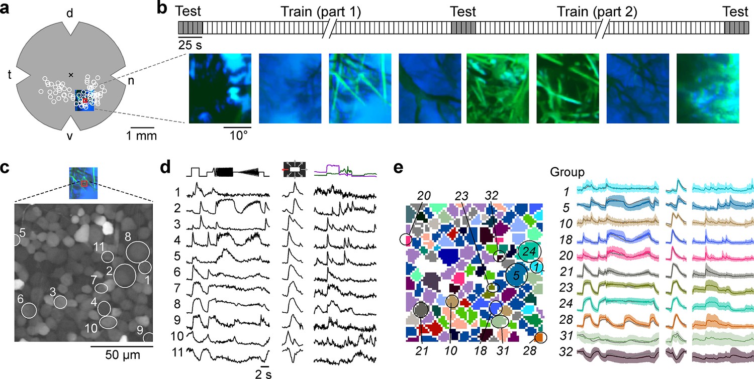
Mouse retinal ganglion cells (RGCs) display diverse responses to a natural movie stimulus.
(a) Illustration of a flat-mounted retina, with recording fields (white circles) and stimulus area centred on the red recording field indicated (cross marks optic disc; d, dorsal; v, ventral; t, temporal; n, nasal). (b) Natural movie stimulus structure (top) and example frames (bottom). The stimulus consisted of 5 s clips taken from UV-green footage recorded outside (Qiu et al., 2021), with 3 repeats of a 5-clip test sequence (highlighted in grey) and a 108-clip training sequence (see Methods). (c) Representative recording field (bottom; marked by red square in (a)) showing somata of ganglion cell layer (GCL) cells loaded with Ca2+ indicator OGB-1. (d) Ca2+ responses of exemplary RGCs (indicated by circles in (c)) to chirp (left), moving bar (centre), and natural movie (right) stimulus. (e) Same recording field as in (c) but with cells colour-coded by functional RGC group (left; see Methods and Baden et al., 2016) and group responses (coloured, mean ± SD across cells; trace of example cells in (d) overlaid in black).
Figure 1—figure supplement 1
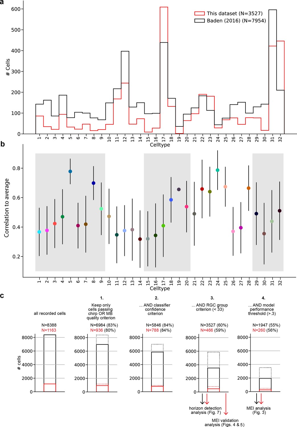
Additional information about the dataset, model performance, and response quality filtering pipeline.
(a) Distribution across cell types for this dataset, and for the dataset described in Baden et al., 2016, which was the basis for our classifier (Qiu et al., 2023). (b) Mean ± SD of model performance, evaluated as correlation between model prediction and retinal ganglion cell (RGC) response on the 25 s long test sequence, averaged across three repetitions of the test sequence, for each cell type. (c) Response quality, RGC group assignment, and model performance filtering pipeline showing the consecutive steps and the fraction of cells remaining after each step. Black bars and numbers indicate cells from all experiments (i.e. all RGCs for which we recorded chirp, moving bar [MB], and movie responses), red bars and numbers indicate the subset of cells recorded in the maximally exciting input (MEI) validation experiments (i.e. those RGCs for which we additionally recorded MEI stimuli responses). Dotted bars indicate the number of cells before the current filtering step. The filtering steps were as follows: (1) Keep only cells that pass the chirp OR MB quality criterion . (2) Keep only cells that the classifier assigns to a group with confidence ≥0.25. (3) Keep only cells assigned to a ganglion cell group (groups 1–32; groups 33–46 are amacrine cell groups). (4) Keep only cells with sufficiently high model performance All cells passing steps 1–3 were included in the horizon detection analysis (Figure 7); all cells passing steps 1–4 were included in the MEI analysis (Figure 3); the ‘red’ cells passing steps 1–4 were included in the MEI validation analysis (Figure 4). All quality criteria are described in the Methods section.
Figure 2
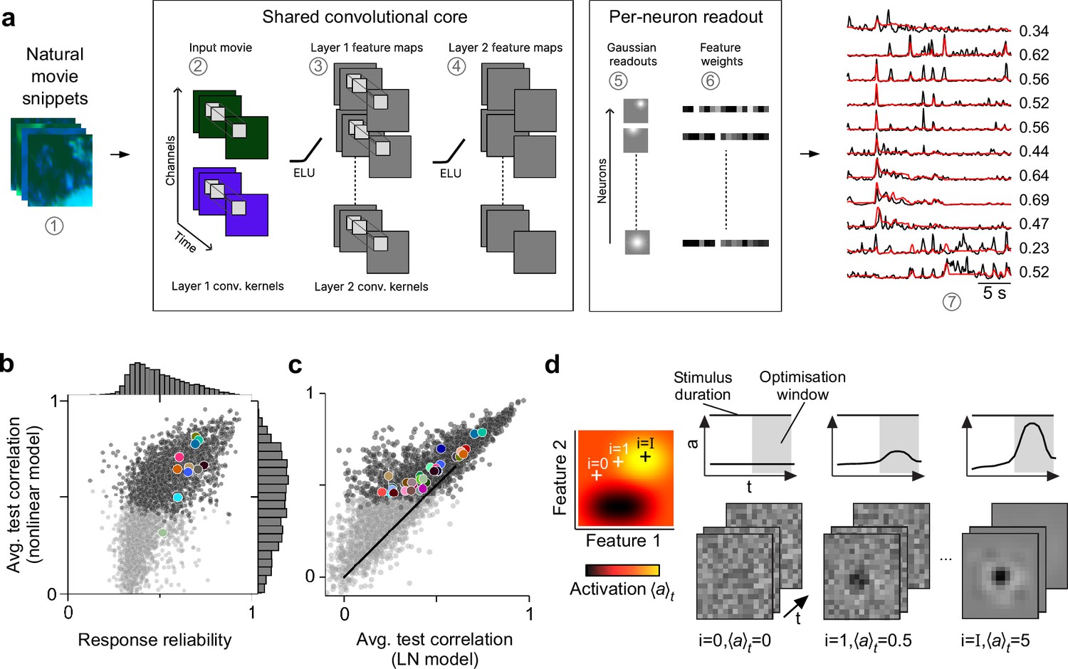
Convolutional neural network (CNN) model captures diverse tuning of retinal ganglion cell (RGC) groups and predicts maximally exciting inputs (MEIs).
(a) Illustration of the CNN model and its output. The model takes natural movie clips as input (1), performs 3D convolutions with space-time separable filters (2) followed by a nonlinear activation function (ELU; 3) in two consecutive layers (2–4) within its core, and feeds the output of its core into a per-neuron readout. For each RGC, the readout convolves the feature maps with a learned RF modelled as a 2D Gaussian (5), and finally feeds a weighted sum of the resulting vector through a softplus nonlinearity (6) to yield the firing rate prediction for that RGC (7). Numbers indicate averaged single-trial test set correlation between predicted (red) and recorded (black) responses. (b) Test set correlation between model prediction and neural response (averaged across three repetitions) as a function of response reliability (see Methods) for N=3527 RGCs. Coloured dots correspond to example cells shown in Figure 1c–e. Dots in darker grey correspond to the N=1947 RGCs that passed the model test correlation and movie response quality criterion (see Methods and Figure 1—figure supplement 1). (c) Test set correlation (as in (b)) of CNN model vs. test set correlation of an LN model (for details, see Methods). Coloured dots correspond to means of RGC groups 1–32 (Baden et al., 2016). Dark and light grey dots as in (b). (d) Illustration of model-guided search for MEIs. The trained model captures neural tuning to stimulus features (far left; heat map illustrates landscape of neural tuning to stimulus features). Starting from a randomly initialised input (second from left; a 3D tensor in space and time; only one colour channel illustrated here), the model follows the gradient along the tuning surface (far left) to iteratively update the input until it arrives at the stimulus (bottom right) that maximises the model neuron’s activation within an optimisation time window (0.66 s, grey box, top right).
Figure 3 with 2 supplements
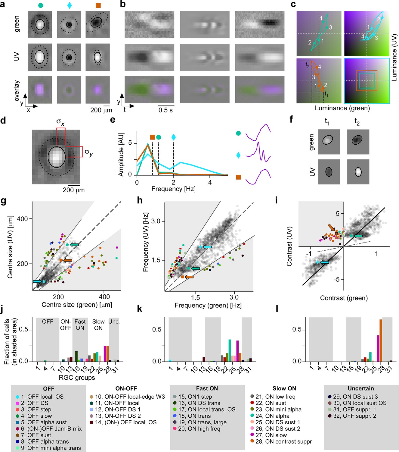
Spatial, temporal, and chromatic properties of maximally exciting inputs (MEIs) differ between retinal ganglion cell (RGC) groups.
(a) Spatial component of three example MEIs for green (top), UV (middle), and overlay (bottom). Solid and dashed circles indicate MEI centre and surround fit, respectively. For display, spatial components in the two channels were re-scaled to a similar range and displayed on a common grey-scale map ranging from black for to white for , i.e., symmetric about 0 (grey). (b) Spatiotemporal (y–t) plot for the three example MEIs (from (a)) at a central vertical slice for green (top), UV (middle), and overlay (bottom). Grey-scale map analogous to (a). (c) Trajectories through colour space over time for the centre of the three MEIs. Trajectories start at the origin (grey level); direction of progress indicated by arrow heads. Bottom right: Bounding boxes of the respective trajectory plots. (d) Calculation of MEI centre size, defined as +, with and the s.d. in horizontal and vertical direction, respectively, of the difference-of-Gaussians (DoG) fit to the MEI. (e) Calculation of MEI temporal frequency: Temporal components are transformed using fast Fourier transform, and MEI frequency is defined as the amplitude-weighted average frequency of the Fourier-transformed temporal component. (f) Calculation of centre contrast, which is defined as the difference in intensity at the last two peaks (indicated by and , respectively, in (c)). For the example cell (orange markers and lines), green intensity decreases, resulting in OFF contrast, and UV intensity increases, resulting in ON contrast. (g) Distribution of green and UV MEI centre sizes across N=1613 cells (example MEIs from (a–c) indicated by arrows; symbols as shown on top of (a)). 95% of MEIs were within an angle of ±8° of the diagonal (solid and dashed lines); MEIs outside of this range are coloured by cell type. (h) As (g) but for distribution of green and UV MEI temporal frequency. 95% of MEIs were within an angle of ±11.4° of the diagonal (solid and dashed lines). (i) As (g) but for distribution of green and UV MEI centre contrast. MEI contrast is shifted away from the diagonal (dashed line) towards UV by an angle of 33.2° due to the dominance of UV-sensitive S-opsin in the ventral retina. MEIs at an angle >45° occupy the upper left, colour-opponent (UVON-greenOFF) quadrant. (j, k) Fraction of MEIs per cell type that lie outside the angle about the diagonal containing 95% of MEIs for centre size and temporal frequency. Broad RGC response types indicated as in Baden et al., 2016. (l) Fraction of MEIs per cell type in the upper-left, colour-opponent quadrant for contrast.
Figure 3—figure supplement 1
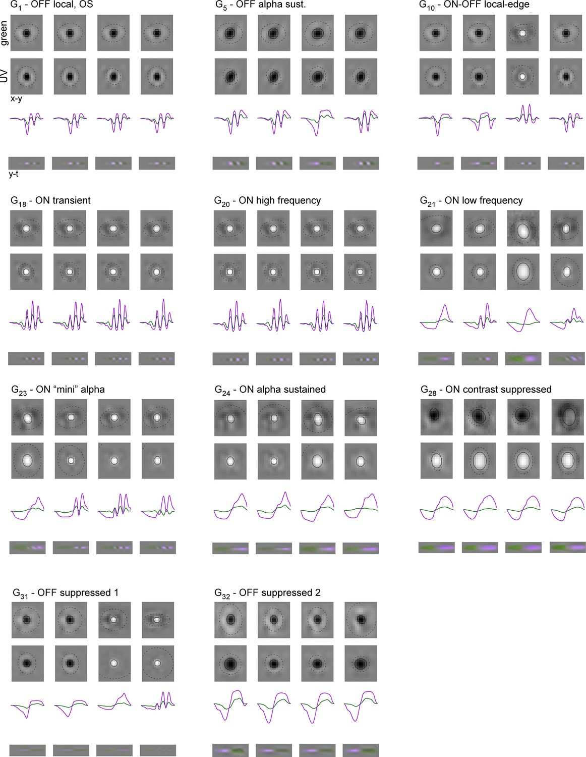
Example maximally exciting inputs (MEIs) for example cell types.
Rows in each panel as in Figure 4a.
Figure 3—figure supplement 2
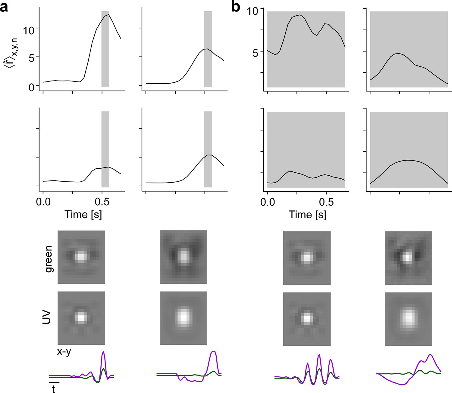
Illustration of how different time windows for optimisation affect maximally exciting input (MEI) temporal properties.
(a) MEIs (bottom panels) and model neuron responses (top panels) for a short optimisation window of 2 frames (≈0.066s, indicated by grey shaded area). The top row shows the responses of a more transient retinal ganglion cell (RGC) to its own MEI (left stimulus) and to the MEI of a more sustained RGC (right stimulus). The bottom row shows the responses of the more sustained RGC to its own MEI (right stimulus) and to the MEI of the more transient RGC (right stimulus). (b) MEIs (bottom panels) and model neuron responses (top panels) for a longer optimisation window of 20 frames (≈0.66s, indicated by grey shaded area) as used throughout the paper. The top row shows the responses of a more transient RGC to its own MEI (left stimulus) and to the MEI of a more sustained RGC (right stimulus). The bottom row shows the responses of the more sustained RGC to its own MEI (right stimulus) and to the MEI of the more transient RGC (right stimulus). Same cells as in (a).
Figure 4 with 1 supplement
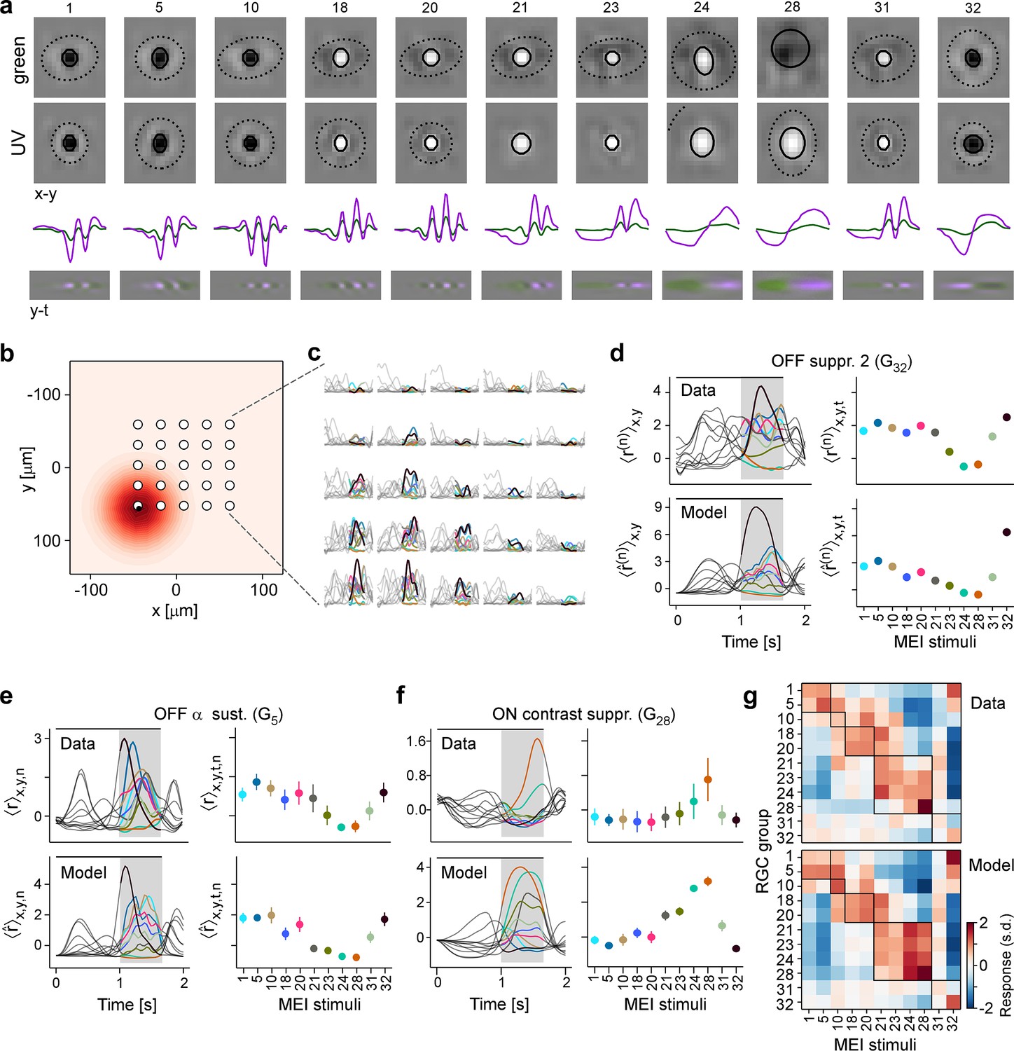
Experiments confirm maximally exciting inputs (MEIs) predicted by model.
(a) MEIs shown during the experiment, with green and UV spatial components (top two rows), as well as green and UV temporal components (third row) and a spatiotemporal visualisation (fourth row). For display, spatial components in the two channels were re-scaled to a similar range and displayed on a common grey-scale map ranging from black for to white for , i.e., symmetric about 0 (grey). Relative amplitudes of UV and green are shown in the temporal components. (b) Illustration of spatial layout of MEI experiment. White circles represent 5 × 5 grid of positions where MEIs were shown; red shading shows an example RF estimate of a recorded G32 retinal ganglion cell (RGC), with black dot indicating the RF centre position (Methods). (c) Responses of example RGC from (b) to the 11 different MEI stimuli at 25 different positions. (d) Recorded [top, ] and predicted [bottom, ] responses to the 11 different MEIs for example RGC from (b, c). Left: Responses are averaged across the indicated dimensions x, y (different MEI locations); black bar indicates MEI stimulus duration (from 0 to 1.66 s), grey rectangle marks optimisation time window (from 1 to 1.66 s). Right: Response to different MEIs, additionally averaged across time (t; within optimisation time window). (e, f) Same as in (d), but additionally averaged across all RGCs () of G5 (N=6) (e) and of G28 (N=12) (f). Error bars show SD across cells. (g) Confusion matrix, each row showing the z-scored response magnitude of one RGC group (averaged across all RGCs of that group) to the MEIs in (a). Confusion matrix for recorded cells (top; ‘Data') and for model neurons (bottom; ‘Model'). Black squares highlight broad RGC response types according to Baden et al., 2016: OFF cells, (G1,5) ON-OFF cells (G10), fast ON cells (G18,20), slow ON (G21,23,24) and ON contrast suppressed (G28) cells, and OFF suppressed cells (G31,32).
Figure 4—figure supplement 1
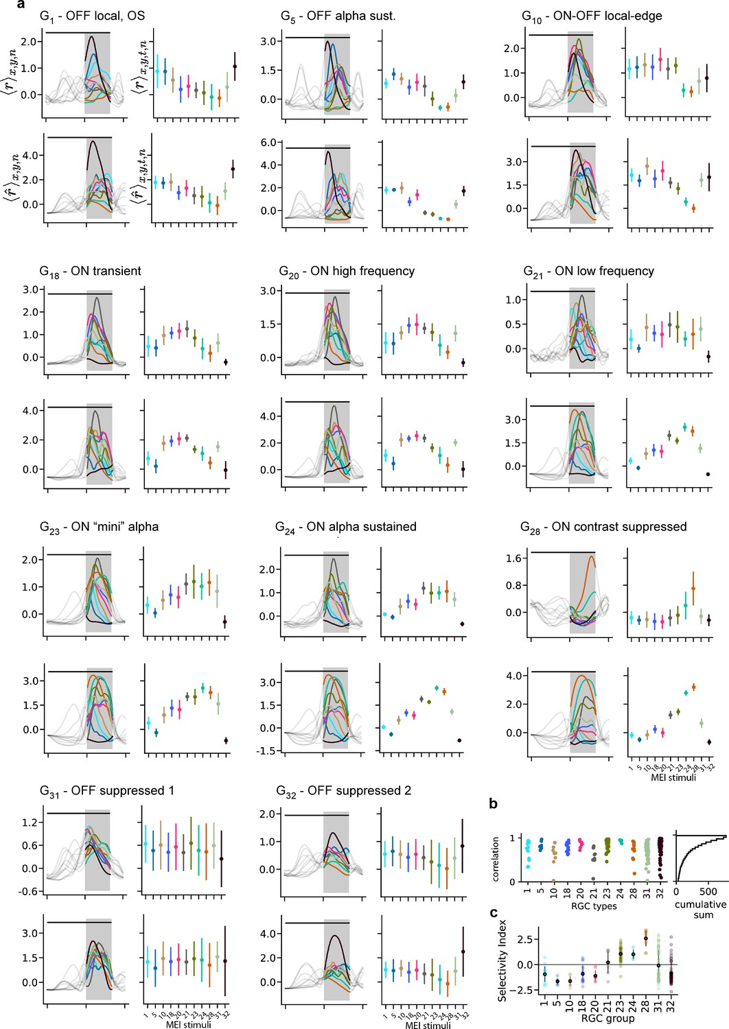
Recorded and predicted responses of example RGC groups to the MEI stimuli.
(a) Recorded (top, ) and predicted (bottom, ) responses to the 11 different maximally exciting inputs (MEIs) for all example cell types. Left: Responses are averaged across the indicated dimensions x, y, n: different MEI locations (x, y) and retinal ganglion cells (RGCs) in a group (n); black bar indicates stimulus duration (from 0 to 1.66 s), grey rectangle marks optimisation time window (from 1 to 1.66 s). Right: Responses to different MEIs, additionally averaged across time (t) within the optimisation time window. Error bars indicate SD across cells. (b) Correlation between the measured and predicted response magnitudes to the MEI stimuli per example cell type. Cumulative histogram is across all N=788 cells; 50% of cells have a correlation between measured and predicted response magnitude of ≥0.8. (c) Mean ± SD of selectivity index (see Methods) for the example cell groups, indicating the difference in response to MEI 28 vs. the average response to all other MEIs in units of standard deviation of the response.
Figure 5
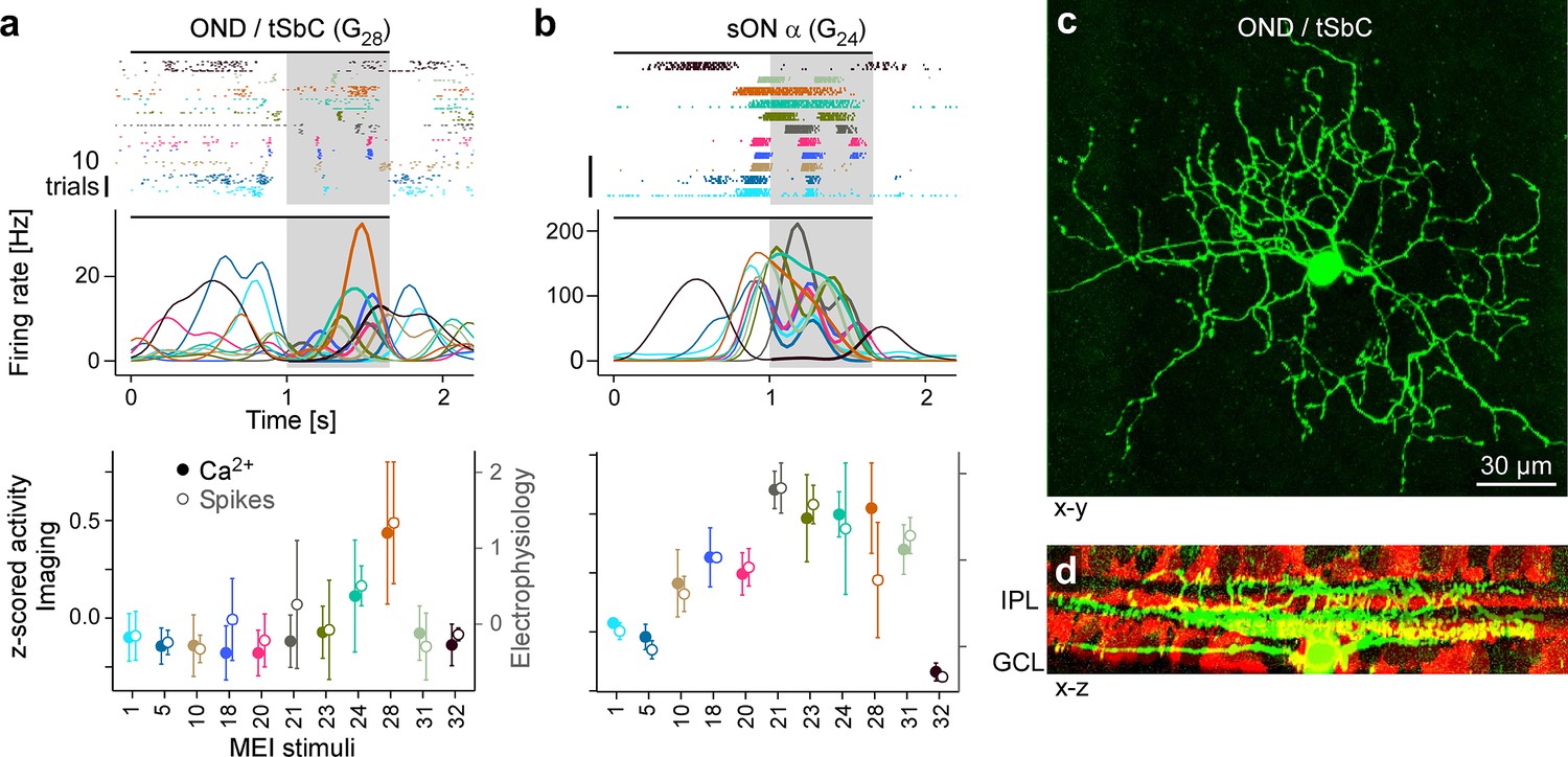
Electrical single-cell recordings of responses to maximally exciting input (MEI) stimuli confirm chromatic selectivity of transient suppressed-by-contrast (tSbC) retinal ganglion cells (RGCs).
(a) Spiking activity (top, raster plot; middle, estimated firing rate) of an OND RGC in response to different MEI stimuli (black bar indicates MEI stimulus duration; grey rectangle marks optimisation time window, from 1 to 1.66 s). Bottom: z-scored activity as a function of MEI stimulus, averaged across cells (solid circles w/ left y-axis, from Ca2+ imaging, N=11 cells; open circles w/ right y-axis, from electrical spike recordings, N=4). Error bars show SD across cells. Colours as in Figure 4. (b) Like (a) but for a sustained ON cell (G24; N=4 cells, both for electrical and Ca2+ recordings). (c) Different ON delayed (OND/tSbC, G28) RGC (green) dye-loaded by patch pipette after cell-attached electrophysiology recording (z-projection; x–y plane). (d) Cell from (c, green) as side projection (x–z), showing dendritic stratification pattern relative to choline-acetyltransferase (ChAT) amacrine cells (tdTomato, red) within the inner plexiform layer (IPL).
Figure 6 with 1 supplement
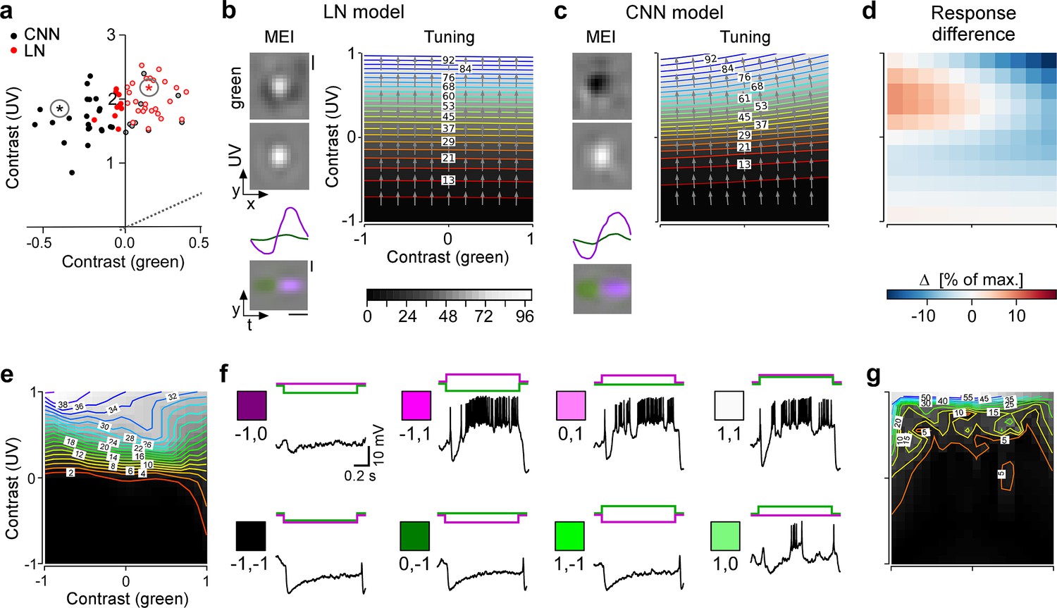
Chromatic contrast selectivity of G28 retinal ganglion cells (RGCs) derives from a nonlinear transformation of stimulus space.
(a) Distribution of green and UV maximally exciting input (MEI) centre contrast for a linear-nonlinear (LN) model (red) and a nonlinear convolutional neural network (CNN) model (black). Colour-opponent cells highlighted by filled marker. (b, c) Left: MEIs for an example cell of RGC group G28, generated with the LN model (b) or the CNN model (c). The cell’s MEI centre contrast for both models is marked in (a) by asterisks. Right: Respective tuning maps of example model neuron in chromatic contrast space. Contour colours and background greys represent responses in % of maximum response; arrows indicate the direction of the response gradient across chromatic contrast space. The tuning maps were generated by evaluating the model neurons on stimuli that were generated by modulating the contrast of the green (x-axis) and UV (y-axis) component of the MEI. In these plots, the original MEI is located at (–1, 1). More details in the Methods section. (d) Difference in response predicted between LN and CNN model (in % of maximum response). (e) Contour plot as in (b, c) but of activity vs. green and UV contrast for an example transient suppressed-by-contrast (tSbC) G28 RGC measured in whole-cell current-clamp mode. Labels on the contour plot indicate spike count along isoresponse curves. (f) Traces are examples of responses at the 8 extremes of –100%, 0, or 100% contrast in each colour channel. Scale bars: (b), vertical 200 µm, horizontal 0.5 s; MEI scaling in (c) as in (b). (g) Same as (e) for a second example tSbC RGC.
Figure 6—figure supplement 1
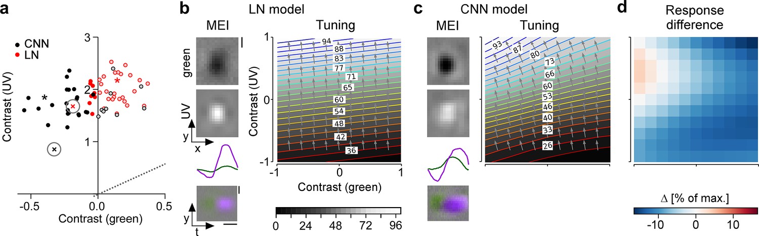
Both LN and CNN model predict colour-opponency for a strongly colour-opponent G_{28} RGC.
(a) Distribution of green and UV maximally exciting input (MEI) centre contrast for a linear-nonlinear (LN) model (red) and a convolutional neural network (CNN) model (black); from Figure 6a. (b, c) Left: MEIs for a second example cell of retinal ganglion cell (RGC) group G28, generated with the LN model (b) or the CNN model (c). The cell’s MEI centre contrast for both models is marked in (a) by cross. Right: Respective tuning maps of example neuron in chromatic contrast space. Colours represent responses in % of maximum response; arrows indicate the direction of the gradient across chromatic contrast space. (d) Difference in response between LN and CNN model (in % of maximum response). Scale bars: (b), vertical 200 µm, horizontal 0.5 s; MEI scaling in (c) same as in (b).
Figure 7 with 3 supplements
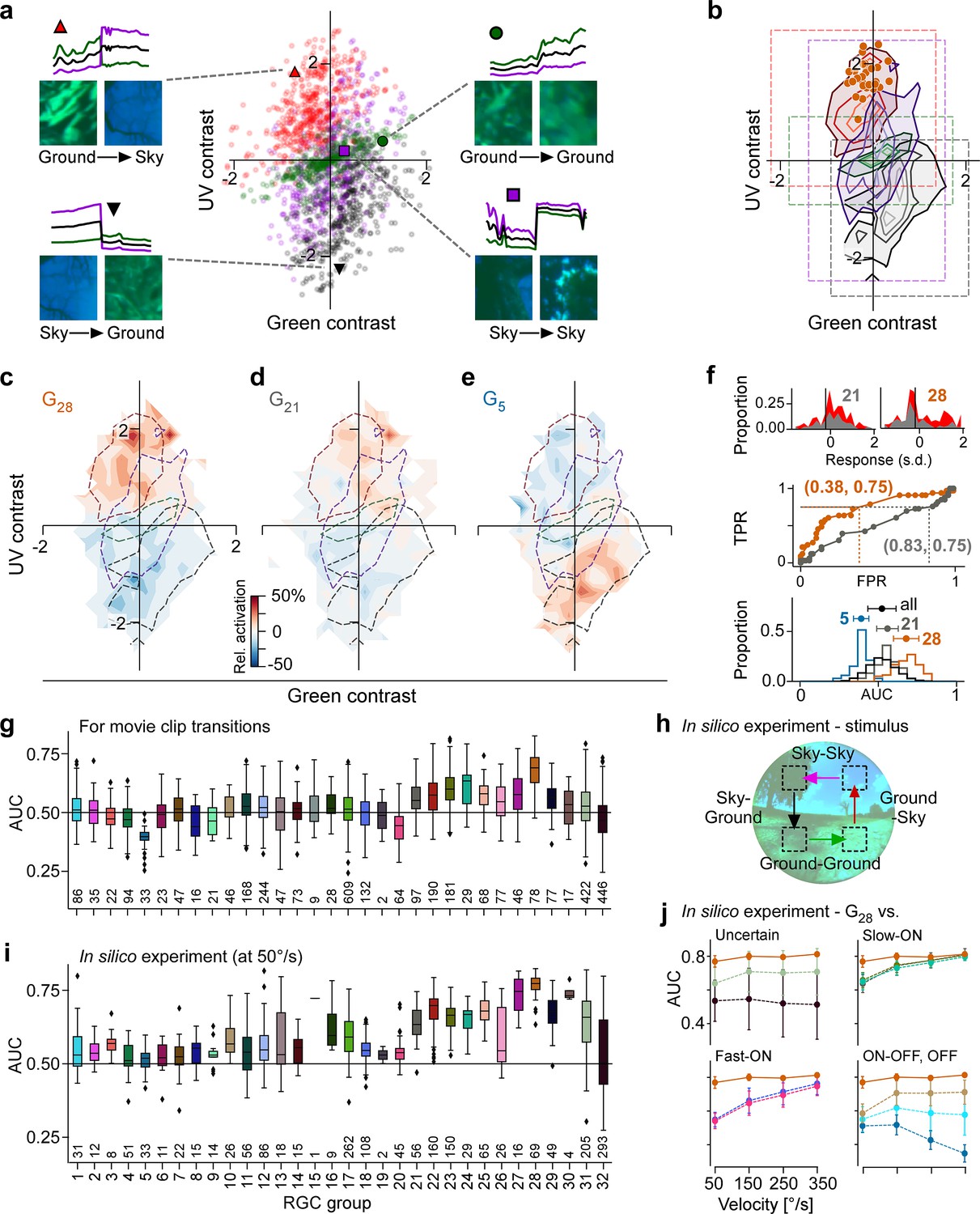
Chromatic contrast tuning allows detection of ground-to-sky transitions.
(a) Distribution of green and UV contrasts of all movie inter-clip transitions (centre), separately for the four transition types, for each of which an example is shown: ground-to-sky (N=525, top left, red triangle), ground-to-ground (N=494, top right, green disk), sky-to-ground (N=480, bottom left, black downward triangle), and sky-to-sky (N=499, bottom right, purple square). Images show last and first frame of pre- and post-transition clip, respectively. Traces show mean full-field luminance of green and UV channels in last and first 1 s of pre- and post-transition clip. Black trace shows luminance averaged across colour channels. (b) Distributions as in (a), but shown as contours indicating isodensity lines of inter-clip transitions in chromatic contrast space. Density of inter-clip transitions was estimated separately for each type of transition from histograms within 10 × 10 bins that were equally spaced within the coloured boxes. Four levels of isodensity for each transition type shown, with density levels at 20% (outermost contour, strongest saturation), 40%, 60%, and 80% (innermost contour, weakest saturation) of the maximum density observed per transition: 28 sky-to-ground (black), 75 ground-to-ground (green), 42 sky-to-sky (purple), and 45 ground-to-sky (red) transitions per bin. Orange markers indicate locations of N=36 G28 maximally exciting inputs (MEIs) in chromatic contrast space (Figure 3i). (c) Tuning map of G28 retinal ganglion cells (RGCs) (N=78), created by averaging the tuning maps of the individual RGCs, overlaid with outermost contour lines from (b) (Figure 7—figure supplement 2). (d, e) Same as (c) for G21 ((g), N=97) and G5 ((h), N=33). (f) Top: Illustration of receiver operating characteristic (ROC) analysis for two RGCs, a G21 (left) and a G28 (right). For each RGC, responses to all inter-clip transitions were binned, separately for ground-to-sky (red) and all other transitions (grey). Middle: Sliding a threshold across the response range, classifying all transitions with response as ground-to-sky, and registering the false-positive rate (FPR) and true-positive rate (TPR) for each threshold yields an ROC curve. Numbers in brackets indicate (FPR, TPR) at the threshold indicated by vertical line in histograms. Bottom: Performance for each cell, quantified as area under the ROC curve (AUC), plotted as distribution across AUC values for all cells (black), G21 (grey), G5 (blue), and G28 (orange); AUC mean ± SD indicated as dots and horizontal lines above histograms. (g) Boxplot of AUC distributions per cell type. Boxes extend from first quartile () to third quartile () of the data; line within a box indicates median, whiskers extend to the most extreme points still within [, ], IQR = inter-quartile range. Diamonds indicate points outside this range. All plot elements (upper and lower boundaries of the box, median line, whiskers, diamonds) correspond to actual observations in the data. Numbers of RGCs for each type are indicated in the plot. (h) Illustration of stimulus with transitions with (Sky-Ground, Ground-Sky) and without (Sky-Sky, Ground-Ground) context change at different velocities (50, 150, 250, and 350 °/s) used in in silico experiments in (i, j). (i) Like (g) but for model cells and stimuli illustrated in (h) at 50/s (see (h)). (j) AUC as function of transition velocity for G28 (orange) vs. example RGC groups (‘Uncertain', G31,32; Slow-ON, G21,23,24; Fast-ON, G18,20; ON-OFF, G10; OFF, G1,5).
Figure 7—figure supplement 1
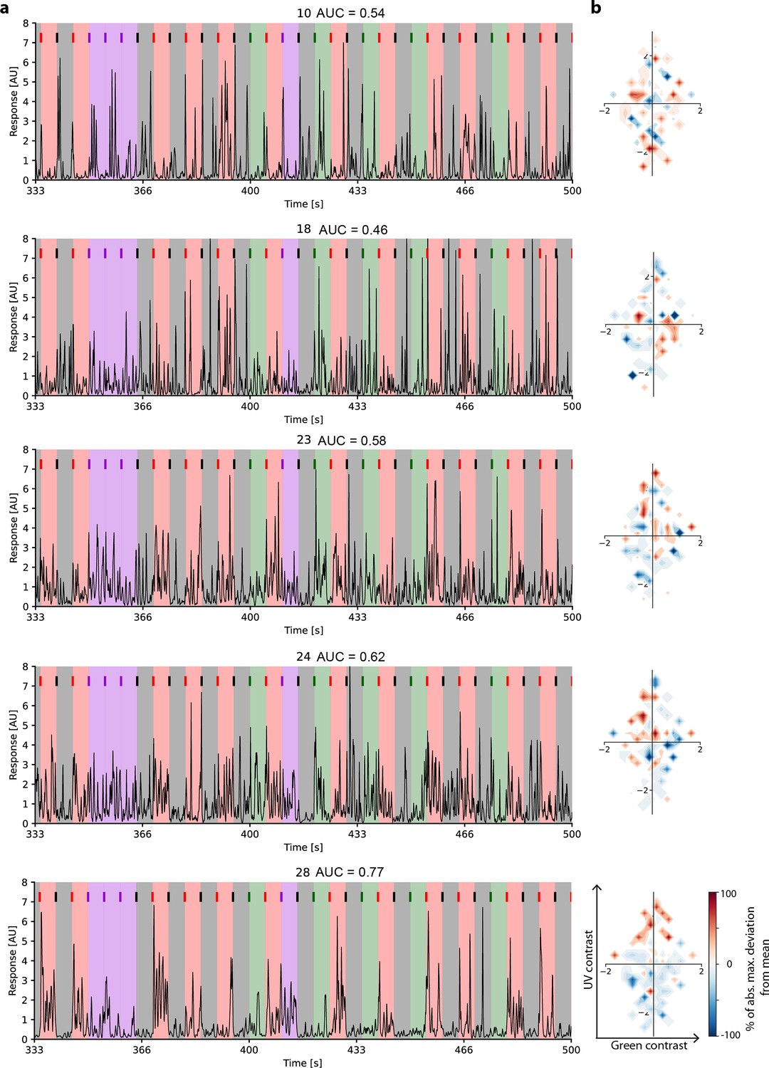
Example response traces to inter-clip transitions with and without context changes.
(a) Traces of example cells of different cell groups (G10, G18, G23, G24, G28) from a single recording field, responding to 33 (of 122) inter-clip transitions. Inter-clip transitions are colour-coded by transition type (red: ground-to-sky, purple: sky-to-sky, green: ground-to-ground, black: sky-to-ground). (b) The resulting tuning maps in chromatic contrast space.
Figure 7—figure supplement 2
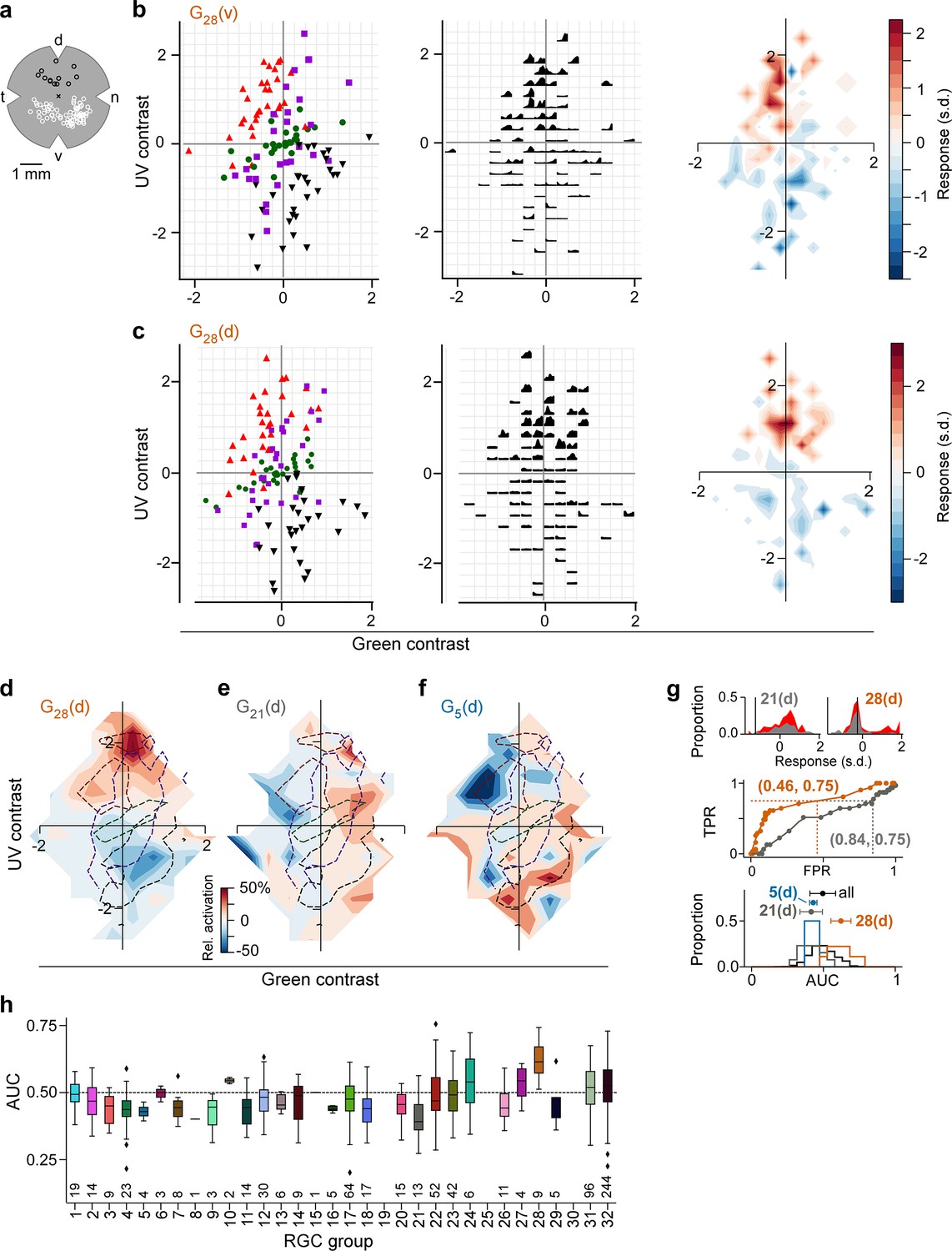
Chromatic contrast tuning in the dorsal retina allows detection of ground-to-sky transitions.
(a) Illustration of a flat-mounted retina, with recording fields in the dorsal (black circles) and ventral (white circles) retina (cross marks optic disc; d, dorsal; v, ventral; t, temporal; n, nasal). (b) Left: Distribution of green and UV contrasts of N=122 inter-clip transitions seen by a ventral group 28 (G28) RGC, coloured by transition type (red triangle, ground-to-sky; green disk, ground-to-ground; black downward triangle, sky-to-ground; purple square, sky-to-sky). Middle: Responses of example RGC in the 1 s following an inter-clip transition, averaged across transitions within the bins indicated by the grid. Right: Responses transformed into a tuning map by averaging within bins as defined by grid. Left: Responses are z-scored (, ). (c) Like (b) but for a dorsal G28 RGC. (d) Tuning map of N=9 dorsal G28 RGCs, created by averaging the tuning maps of the individual RGCs. (e) Same as (d) for N=13 G21 RGCs. (f) Same as (d) for N=4 G5 RGCs. (g) Top: Illustration of receiver operating characteristic (ROC) analysis for two dorsal RGCs, a G21 (left) and a G28 (right). For each RGC, responses were binned to all inter-clip transitions, separately for ground-to-sky (red) and all other transitions (grey). Middle: Sliding a threshold across the response range, classifying all transitions with response as ground-to-sky, and registering the false-positive rate (FPR) and true-positive rate (TPR) for each threshold yields an ROC curve (middle). Numbers in brackets indicate (FPR, TPR) at the threshold indicated by black vertical line in histogram plots. Bottom: We evaluated performance for each cell as the area under the ROC curve (AUC), and plotted the distribution across AUC values for all cells (black), for G5 (blue), for G21 (grey), and for G28 (orange). Among the dorsal RGCs, G28 RGCs achieved the highest AUC on average (mean±SD AUC, G28 (N=9 cells): 0.62±0.07; all other groups (N=720): 0.49±0.09, , bootstrapped 95% confidence interval, Cohen’s two-sample permutation test G28 vs. all other groups (see Methods): with 100,000 permutations; next-best performing G24 (N=6): 0.54±0.12, bootstrapped 95% confidence interval, Cohen’s two-sided -test G28 vs. G24: with 100,000 permutations (not significant). AUC mean ± SD indicated as dots and horizontal lines above histograms. (h) Boxplot of AUC distributions per cell type (dorsal). The box extends from the first quartile () to the third quartile () of the data; the line within a box indicates the median. The whiskers extend to the most extreme points still within [, ], IQR =inter-quartile range. Diamonds indicate points outside this range. All elements of the plot (upper and lower boundaries of the box, median line, whiskers, diamonds correspond to actual observations in the data. Numbers of RGCs for each type are indicated in the plot.
Figure 7—figure supplement 3
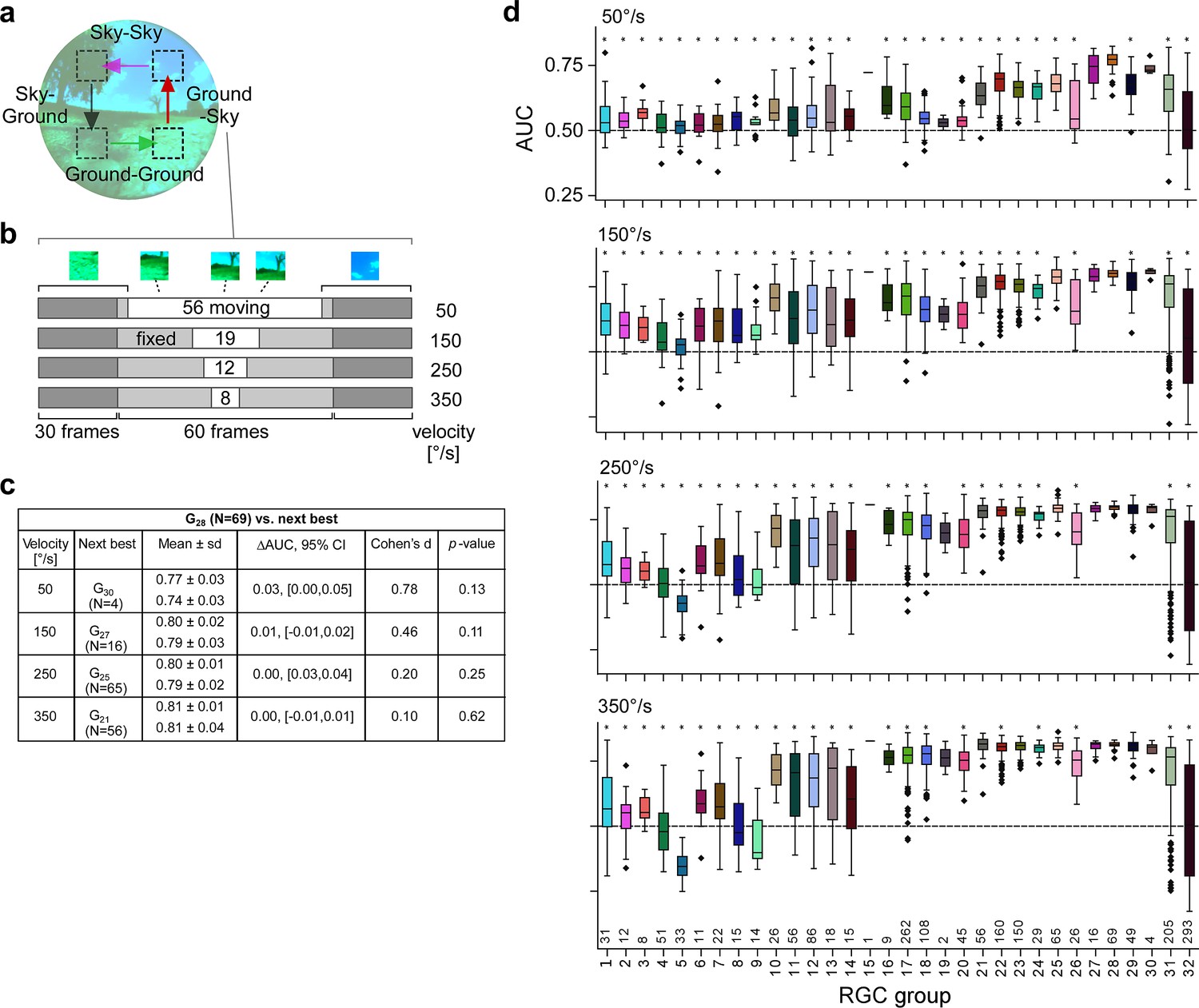
Simulations predict tSbC cells robustly detect context changes across different speeds.
(a) Illustration transition stimulus paradigm (from Figure 7h). (b) Structure of stimuli for different velocities, using a ground-to-sky transition as an example. (c) Statistics of the area under the receiver operating characteristic (ROC) curve (AUC) for the sky-ground detection task in the simulation for different velocities (G28 vs. the next-best retinal ganglion cell [RGC] group). Columns (from left): mean ± standard deviation of AUC values (top: G28; bottom: the respective best next RGC type); difference in mean AUC and corresponding bootstrapped 95% confidence intervals; Cohen’s d and p-value of a two-sample permutation test with 100,000 repeats. (d) Boxplots of AUC distributions per cell type for the different velocities (plots like in Figure 7g and j).
Additional files
Download links
A two-part list of links to download the article, or parts of the article, in various formats.
Downloads (link to download the article as PDF)
Open citations (links to open the citations from this article in various online reference manager services)
Cite this article (links to download the citations from this article in formats compatible with various reference manager tools)
A chromatic feature detector in the retina signals visual context changes
eLife 13:e86860.
https://doi.org/10.7554/eLife.86860


