Judging the difficulty of perceptual decisions
- Zuckerman Mind Brain Behavior Institute, Columbia University, United States
- Department of Neuroscience, Columbia University, United States
- Kavli Institute for Brain Science, Columbia University, United States
- Howard Hughes Medical Institute, Columbia University, United States
Figures
Figure 1

Reaction time color and difficulty judgment tasks (Experiment 1).
(a) Schematic of the color judgment task. Participants judged the dominant color of a single random dot stimulus consisting of blue and yellow dots. (b) Proportion of correct choices (top) and reaction time (bottom) as a function of color strength. Solid lines show the average of fits of a standard drift diffusion model to each participant’s choices and reaction times (RTs). Values of the fit parameters are shown in Supplementary file 1. Data points show mean ± 1 SEM from 20 participants. (c) Schematic of the difficulty judgment task. Participants decided for which of the two stimuli it was easier to judge the dominant color, regardless of whether that stimulus was blue or yellow dominant. (d) Proportion of trials in which stimulus 1 (S1) was chosen as the easier stimulus (top) and RTs (bottom) as a function of the strength of S1 (abscissa) and S2 (colors). Open circles identify conditions where both patches have the same color strength (also plotted in inset). Data points show mean ± 1 SEM from 20 participants.
Figure 2
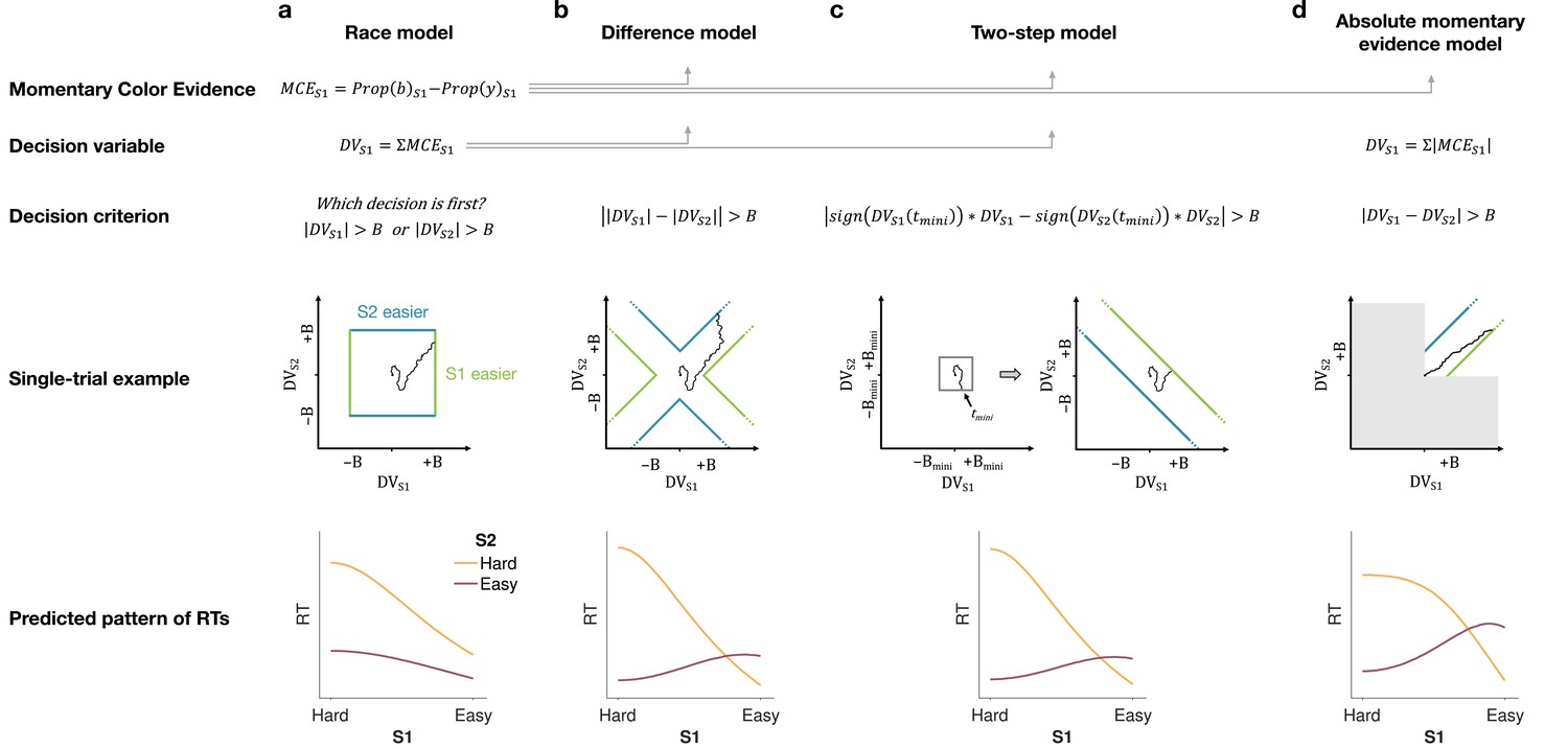
Models of difficulty judgments.
In each model, momentary color evidence (MCE) is obtained simultaneously from each of the two stimuli as the difference in proportion of blue vs. yellow dots on each frame. The models differ in (i) how this momentary evidence is accumulated into a decision variable (second row) and (ii) how the bounds are set for the decision (third row). For each model, an example of a simulation of a single trial (fourth row) is illustrated in the 2D space of the decision variables and for the left (S1) and right (S2) stimuli. Each simulation shows a biased random walk that starts at the origin and terminates when it reaches one of the decision bounds. Decision bounds in green and blue correspond to S1 and S2 being judged the easier decision, respectively. For clarity, all bounds are illustrated as time-independent (although in the model they are allowed to collapse over time). The models predict different patterns of reaction times (RTs; bottom row) for different difficulty combinations of S1 (abscissa) and S2 (magenta = easy, yellow = hard). (a) The race model, (b) the difference model, (c) the two-step model, and (d) the absolute momentary evidence model (gray area is not reachable as all accumulation is positive). See main text for model details.
Figure 3
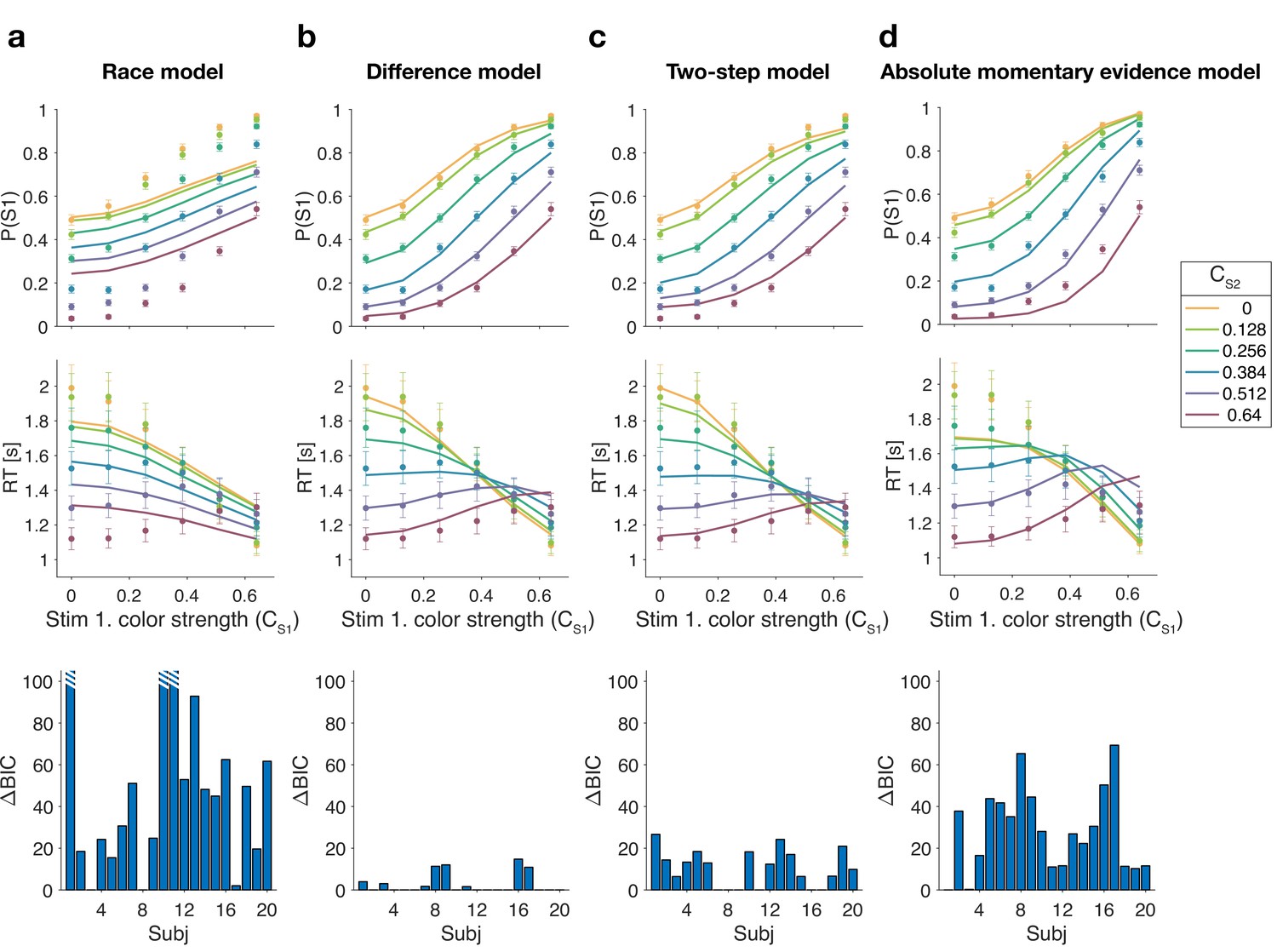
Reaction time difficulty judgment results (Experiment 1).
Fits and model comparisons for (a) The race model, (b) the difference model, (c) the two-step model, and (d) the absolute momentary evidence model. Difficulty choices (top row) are shown as the proportion of trials in which participants chose S1 (left stimulus) as the easier stimulus. Reaction times are shown in the middle row. Data points are averages across participants (mean ± 1 SEM; ). Lines represent model fits. Bottom row: BIC values for each model, relative to BIC value of the winning model for each participant (hatched bars represent values ).
Figure 4
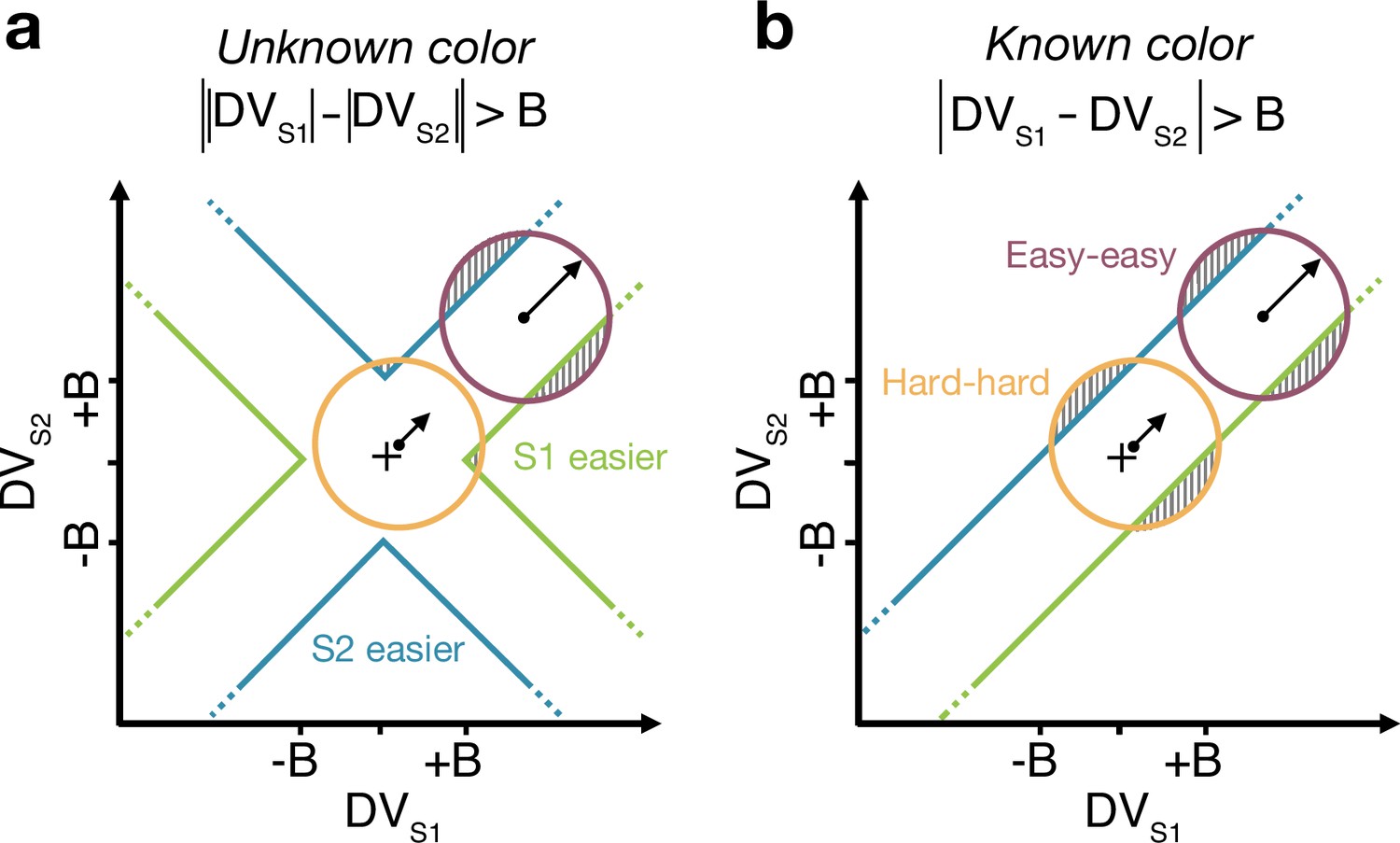
Reaction time task for unknown vs. known color dominance.
(a and b) Schematic illustration of the unknown vs. known color tasks. For each condition, the dispersion of decision variables (DVs) is represented in the 2D space of (abscissa) and (ordinate), assuming a constant noise in the drift diffusion process independent of strength. To provide intuition colored circles show the dispersion expected without absorption at the bounds and represent contours of equal density of the decision variable. Green and blue lines represent decision boundaries (B) for S1 and S2 being easier. (a) In the unknown color condition, the difference model computes the difference between the two absolute DVs. (b) In the known color condition (example shown is for both stimuli blue dominant), the model compares the signed DVs, resulting in a larger region where the DV dispersion crosses the bounds (shaded areas). Thus, when both stimuli are blue-dominant, yellow (negative) evidence for S1 contributes to the decision that S2 is the easier stimulus.
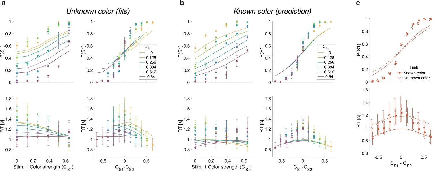
Figure 5
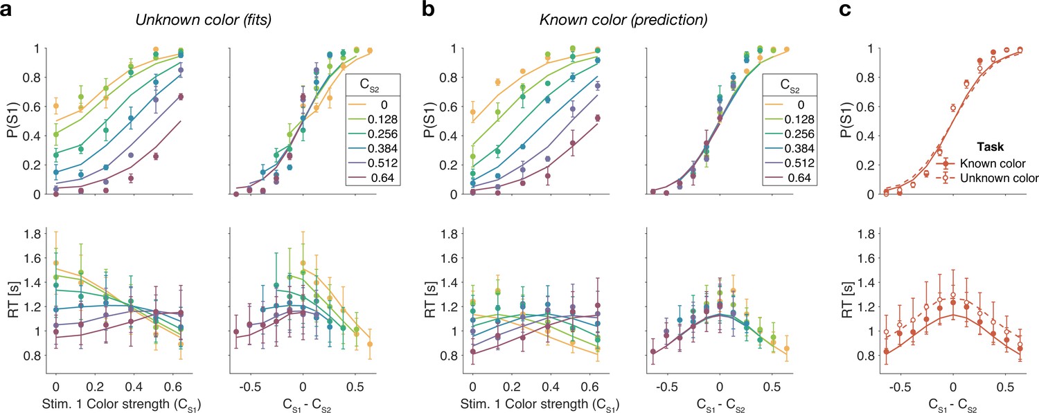
Reaction time task for unknown vs. known color dominance (Experiment 2a).
(a) Unknown color condition. Proportion of S1 choices (top row) and reaction times (bottom row) plotted as a function of strength of S1 (left column) and difference of strengths of the two stimuli (right column). Lines show the fit of the difference model. (b) As (a) for the known color condition. Lines show the predictions of behavior when the color dominance is known (correct sign applied as in Figure 4b) based on the parameters obtained in the fit to (a). (c) Comparison of overall choice performance and reaction times (RTs) in the known vs. unknown color condition as a function of the absolute difference in strength levels (data mean ± 1 SEM across three participants).
Figure 6
Same as Figure 5 but with lines showing the fit of the confidence model to the unknown color condition and predictions for the known color condition.
Figure 7
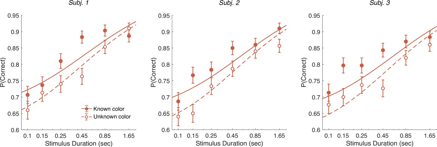
Controlled duration task for unknown vs. known color dominance.
Performance in the controlled duration task for difficulty judgments in the known (solid-red) and unknown color condition (open-red). Participants’ accuracy (mean ± 1 SEM) is shown for each stimulus duration. Here, we exclude trials which had no objective correct answer (i.e., trials in the difficulty task where S1 and S2 had the same strength). Lines illustrate model fits for the six stimulus times used in the experiment. Results are shown for individual participants.
Figure 8
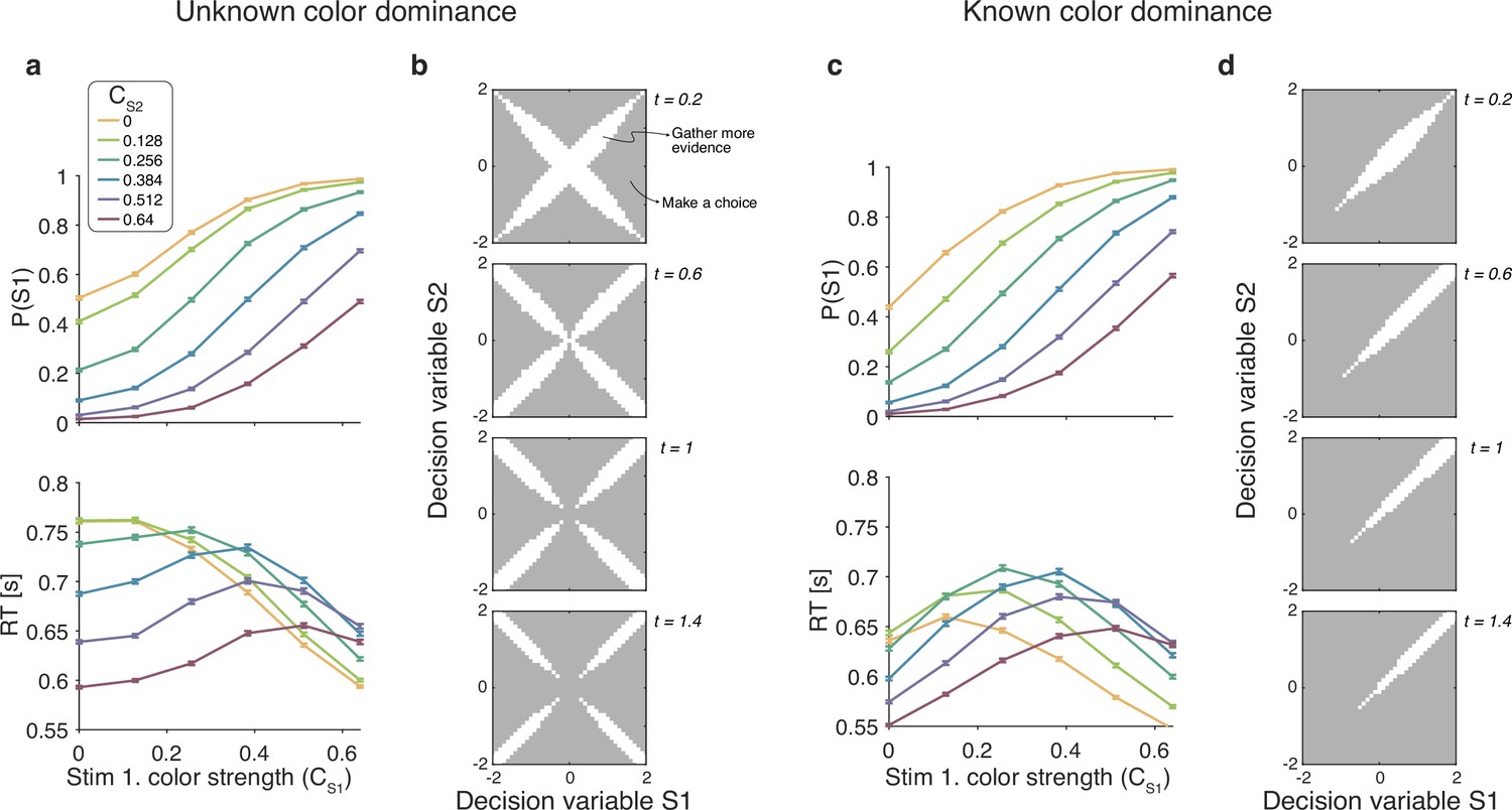
Optimal policy for difficulty decisions.
(a) Choices and response times obtained from simulations of the model that maximizes the rate of correct choices, derived for the reaction time version of the task with unknown color dominance (as in Experiment 1; N=200,000 simulated trials). (b) The optimal decision policy is a deterministic mapping from a belief state to an action. The figure identifies the values of the decision variables for stimuli S1 and S2, for which it is optimal to continue sampling sensory information (shown in white) or commit to a choice (shown in gray). Each panel represents different time within a trial (where the time spent sampling each stimulus is t/2). (c and d) Same as panels (a and b), but for the version of the reaction time task in which the color dominance is known (as in Experiment 2).
Additional files
-
Supplementary file 1
Fit parameter values for drift diffusion model of color judgments (Experiment 1a).
- https://cdn.elifesciences.org/articles/86892/elife-86892-supp1-v1.docx
-
Supplementary file 2
Fit parameter values for race model (Experiment 1).
- https://cdn.elifesciences.org/articles/86892/elife-86892-supp2-v1.docx
-
Supplementary file 3
Fit parameter values for difference model (Experiment 1).
- https://cdn.elifesciences.org/articles/86892/elife-86892-supp3-v1.docx
-
Supplementary file 4
Fit parameter values for two-step model (Experiment 1).
- https://cdn.elifesciences.org/articles/86892/elife-86892-supp4-v1.docx
-
Supplementary file 5
Fit parameter values for absolute momentary evidence model (Experiment 1).
- https://cdn.elifesciences.org/articles/86892/elife-86892-supp5-v1.docx
-
Supplementary file 6
Fit parameter values for difference model in reaction time task (Experiment 2).
- https://cdn.elifesciences.org/articles/86892/elife-86892-supp6-v1.docx
-
Supplementary file 7
Fit parameter values for difference model in controlled duration task (Experiment 2).
The high parameter for subject 2 implies that the decision process was not bounded.
- https://cdn.elifesciences.org/articles/86892/elife-86892-supp7-v1.docx
-
Supplementary file 8
Fit parameter values for confidence model in reaction time task (Experiment 2).
- https://cdn.elifesciences.org/articles/86892/elife-86892-supp8-v1.docx
-
MDAR checklist
- https://cdn.elifesciences.org/articles/86892/elife-86892-mdarchecklist1-v1.docx
-
Source data 1
The raw Matlab data set for all the experiments.
- https://cdn.elifesciences.org/articles/86892/elife-86892-supp9-v1.zip
Download links
A two-part list of links to download the article, or parts of the article, in various formats.
Downloads (link to download the article as PDF)
Open citations (links to open the citations from this article in various online reference manager services)
Cite this article (links to download the citations from this article in formats compatible with various reference manager tools)
Judging the difficulty of perceptual decisions
eLife 12:RP86892.
https://doi.org/10.7554/eLife.86892.3


