Sexual coordination in a whole-brain map of prairie vole pair bonding
Figures
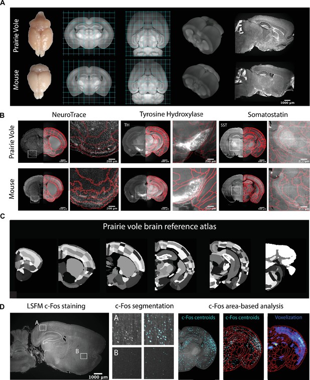
Prairie vole reference brain and atlas generation for automatic c-Fos analysis.
(A) Generation of prairie vole (upper row) and mouse (lower row) reference brains was done with light-sheet fluorescence microscopy (LSFM) imaging. Shown is the top view of both prairie vole and mouse brains after perfusion. Also shown are cross-sections of coronal and horizontal views of prairie vole and mouse reference brains built after the co-registration of nearly 200 brains per species (approximately 190 voles and 150 mice). The prairie vole whole brain was 1.39 times larger than the mouse brain (see Figure 1—figure supplement 1 and Supplementary file 1). Both prairie vole and mouse brains underwent 3D renderization. Also shown are sagittal views of prairie vole and mouse whole-brain fluorescent Nissl (NeuroTrace) staining imaged with LSFM. The scale bar represents a distance of 1,000 μm. (B) Whole-brain staining of both prairie vole (upper row) and mouse (lower row) brains were registered to the reference brain. In red, boundaries of registered mouse reference atlas are plotted onto both prairie vole and mouse reference brains. NeuroTrace, tyrosine hydroxylase (TH), and somatostatin (SST) were registered and overlaid onto the atlases for validation. (C) Coronal sections of the resulting prairie vole atlas after manual validation. Scale bars represent distances of 1,000 μm and 200 μm for whole section and close-up views, respectively. (D) Overview of LSFM prairie vole c-Fos analysis pipeline. Shown in the left panel is a sagittal section of prairie vole c-Fos immunolabeling imaged with LSFM (scale bar represents a distance of 1,000 μm). Shown in the center panel are detailed views of two brain locations immunolabeled with c-Fos and overlaid with the resulting segmentation. Shown in the right panel is an area-based analysis of c-Fos+ cells. All c-Fos+ cell centroids are registered to the prairie vole reference brain and analyzed using the new prairie vole reference atlas. For each brain, a voxel representation is generated of all c-Fos+ cells in the same prairie vole reference space and overlaid with the reference atlas.
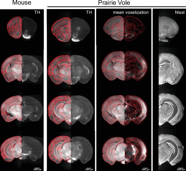
Validation of the prairie vole reference atlas.
Mouse coronal sections (left column) are composed of the mouse reference brain overlaid with atlas boundaries in red on the left and, in the same sections, of tyrosine hydroxylase (TH) immunolabeling on the right. Prairie vole coronal sections are in the right three columns. In the first vole column, coronal brain sections are of the prairie vole reference brain and atlas boundaries in red on the left with TH immunolabeling on the right. In the second vole column, coronal sections are of the prairie vole reference brain and c-Fos+ mean voxelization overlay with atlas boundaries in red. In the third vole column, coronal sections of prairie vole NeuroTrace staining are registered onto the prairie vole reference brain. Scale bars represent a distance of 1,000 μm.
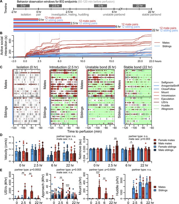
Study design and development of the prairie vole pair bond.
(A) Schematic of the experiment design is shown, where social behaviors (during 1 hr observations, black blocks) and immediate early gene (IEG) expression patterns are compared between mate pairs and siblings across time. (B) Continuous automated tracking is shown for active social interactions (i.e., an index of social investigation and mating) in mate pairs (red lines) and sibling pairs (blue lines). (C) Time courses are shown for specific social behaviors during 1 hr observation windows that correspond to IEG expression, with each row representing one pair. Social behaviors are overlaid onto self-grooming (grey), and ultrasonic vocalizations (USVs, short dark red ticks) are overlaid onto all behaviors. Other behaviors shown include anogenital investigation (light blue), close follows (dark blue), mount (very light red), intromissions (light red), ejaculation (red), huddle (light green), and allogroom (dark green). (D) Plots show group differences (mean ± standard deviation [SD]) in individual activity level (velocity) and movement relative to the partner (net move, positive values indicate movement toward the partner). (E) Group differences (mean ± SD) are shown for vocal behavior (ultrasonic vocalizations [USVs]), proximity seeking (approach), mating (mount), and side-by-side contact (huddle). For (D, E), mate pairs are in red and sibling pairs in blue for dyadic-level behaviors (USVs, mount, and huddle). Females are a lighter hue and males a darker hue for behaviors measured on an individual level (velocity, netmove, approach). T-tests were used to compare mate animals (n = 94) or mate dyads (USVs: n = 48; mount and huddle: n = 47) with sibling animals (n = 96) or sibling dyads (n = 48). Paired t-tests were used to compare female mates (n = 47) with male mates (n = 47). For behaviors with group-level effects, follow-up t-tests were performed for each timepoint (n = 11-12 animals/group or n = 22-24 dyads/group; significance represented by * p<0.05, ** p<0.01, *** p<0.001). Descriptions of vole behaviors are listed in Supplementary file 3.
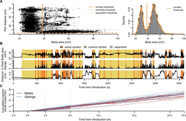
Automated tracking of social behavior states.
(A) Long-term tracking of social states was informed by automated measures of the largest body area, pair activity, and pair distance. On the left, body area is plotted against dyad distance from an exemplar 24 hr mate pair video (10% randomly selected frames from 12 hr of white light). On the right, the density curve for body area reveals a basic threshold for when animals are separated or in physical contact. (B) Traces of body area, video activity, and pair distance are plotted for the first hour of interaction in the exemplar mate pair, along with automated assignments of behavioral states. (C) Cumulative time spent in inactive social contact is shown for up to 22 hr of cohabitation in mate pairs (red lines) and sibling pairs (blue lines).
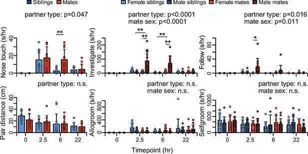
Time course of social behaviors during pairing.
Group differences (mean ± standard deviation [SD]) are shown for appetitive behaviors including nose-to-nose touching, anogenital investigation, and close follows. Group differences (mean ± SD) are also shown for proximity and grooming behaviors including pair distance, allogrooming, and selfgrooming. Mate pairs are in red and sibling pairs are in blue for dyadic-level behaviors (nose touch and pair distance). For individual-level behaviors (investigate, follow, allogroom, and selfgroom), females are shown in lighter hues, and males in darker hues. T-tests were used to compare mate animals (n = 94) or mate dyads (n = 47) with sibling animals (n = 96) or sibling dyads (n = 48). Paired t-tests were used to compare female mates (n = 47) with male mates (n = 47). For behaviors with main effects, follow-up t-tests were performed for each timepoint (n = 11-12 animals/group or n = 22-24 dyads/group; significance represented by * p<0.05, ** p<0.01). Descriptions of vole behaviors are listed in Supplementary file 3.
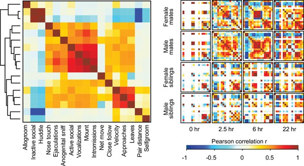
Associations between behavioral states and types of social interaction.
Hierarchical clustering of behavioral measures from Pearson correlations is used to group behavioral states and social interactions into three main clusters (n = 190 animals). These clusters involve close contact (e.g., huddling and allogrooming), mating (e.g., mounts and vocalizations), and appetitive behavior (e.g., approaches and follows). On the right, Pearson correlations are shown among behaviors in subsets based on partner type, sex, and timepoint (n = 11-12 animals/group). Warm and cool colors indicate positive and negative correlation coefficients, respectively. White indicates behaviors with no variation, meaning that coefficients were not calculated (e.g., siblings did not exhibit mating behaviors). Descriptions of vole behaviors are listed in Supplementary file 3.
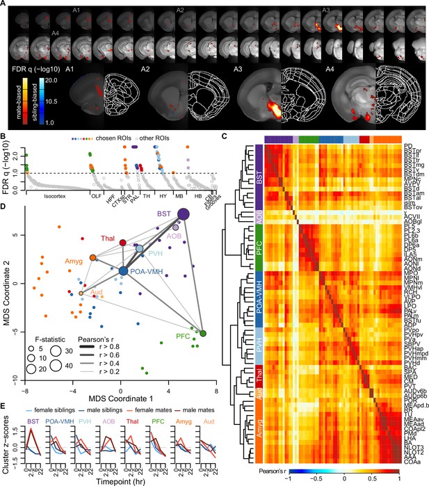
A brain-wide functional network is active during pair bond formation.
(A) Map of bonding-associated voxels is shown in coronal sections (rostral to caudal) spanning the vole brain. Brightness indicates significance levels for comparisons of hypothesized and null generalized linear models (GLMs) to predict c-Fos+ cell counts across 189 vole brain samples. For each voxel, an analysis of variance (ANOVA) test was used to compare null and hypothesized GLMs. False discovery rate (FDR) q-values were computed from the ANOVA results to account for multiple comparisons across voxels (alpha threshold of q = 0.1). Warm colored voxels have higher mean c-Fos+ cell counts in mates (n = 94) compared to siblings (n = 95) (GLM test statistic for partner type > 0). Cool colored voxels have lower mean c-Fos+ cell counts in mates compared to siblings (GLM test statistic for partner type < 0). (B) Identification of significant and mutually exclusive regions of interest (ROIs, n = 68 chosen and 824 total ROIs) is shown sorted by anatomical division and F-statistic. For each ROI, an ANOVA test was used to compare null and hypothesized GLMs. The significance levels of ANOVAs were determined by comparing the observed F-statistic to its null distribution from shuffled data (10,000 permutations). False discovery rate (FDR) q-values were computed to adjust for multiple comparisons acros ROIs (alpha threshold of q = 0.1). Colored symbols for ROIs match their cluster group assignments in (C) and (D). (C) Hierarchical clustering of chosen ROIs (n = 68, permutation tests with FDR q < 0.1) is shown alongside pairwise Pearson correlations of c-Fos+ cell counts. Full ROI names are listed in Supplementary file 4. (D) Multi-dimensional scaling (MDS) coordinate space of the correlations is shown between chosen ROIs (n = 68). The most significant ROIs per cluster are labeled with the symbol size scaled by the F-statistic. Darkness and thickness of connecting lines reflect Pearson correlation coefficients. (E) Time course trajectories of total c-Fos+ cell counts are shown for each cluster. Counts per cluster are scaled across samples with means taken for each experiment group (n = 11-12 animals/group). Red lines represent mates and blue lines represent siblings (females – lighter, males – darker). In (C, D, E), each cluster group is given a label to summarize the most significant ROIs within it. Cluster group labels include ‘BST’ (bed nucleus of the stria terminalus) in dark purple, ‘AOB’ (accessory olfactory bulb) in light purple, ‘PFC’ (prefrontal cortex) in green, ‘POA-VMH’ (preoptic area, ventromedial hypothalamus) in dark blue, ‘PVH’ (paraventricular hypothalamus) in light blue, ‘Thal’ (thalamus) in red, ’Aud’ (auditory cortex) in light orange, and ‘Amyg’ (amygdala) in dark orange.
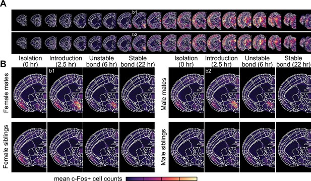
Brain-wide patterns of immediate early gene activation during pairing.
(A) Coronal cross-sections (rostral to caudal) from female (top) and male (bottom) mating pairs are shown for the 2.5 hr timepoint group, with brightness corresponding to the mean voxel c-Fos+ cell counts (n = 12 female and 12 male mates). (B) A representative coronal slice that includes the posterior part of the bed nucleus of the stria terminalis is shown for mate pairs and siblings and separated by timepoint and sex. Brightness corresponds to mean voxel c-Fos+ cell counts per group (n = 11-12 animals/group).
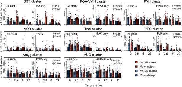
Patterns of immediate early gene expression in brain region clusters.
Counts of c-Fos+ cells are shown for regions of interest (ROIs) associated with pair-bond development (n = 68), organized by hierarchical cluster. For each cluster, the total counts are shown on the right and the most significant ROI (highest F-statistic) is shown on the right. For each ROI, an analysis of variance (ANOVA) test was used to compare null and hypothesized generalized linear models (GLMs). The significance levels of the ANOVAs were determined by comparing the observed F-statistic to its null distribution from shuffled data (10,000 permutations). False discovery rate (FDR) q-values were computed to adjust for multiple comparisons across ROIs (alpha threshold of q = 0.1). Counts are summarized by timepoint, partner type, and sex (mean ± standard deviation [SD], n = 11-12 animals/group). Mate pairs are in red and sibling pairs in blue (females in lighter hues, males in darker hues). Cluster group labels include ‘BST’ (bed nucleus of the stria terminalus), ‘POA-VMH’ (preoptic area, ventromedial hypothalamus), ‘PVH’ (paraventricular hypothalamus), ‘AOB’ (accessory olfactory bulb), ‘Thal’ (thalamus), ‘PFC’ (prefrontal cortex), ‘Amyg’ (amygdala), and ’Aud’ (auditory cortex). Representative ROIs include PD (posterodorsal preoptic nucleus), MPO (medial preoptic area), PVpo (periventricular hypothalamic nucleus, preoptic part), y (nucleus y), BAC (bed nucleus of the anterior commisure), PL5 (prelimbic area layer 5), POR (superior olivary complex, periolivary region), and AUDv6b (ventral auditory area layer 6b).
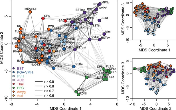
Multi-dimensional structure of brain-wide correlation patterns.
Representations of the first three dimensions of a multi-dimensional scaling (MDS) coordinate space based on Pearson correlations between c-Fos+ cell counts in brain regions of interest (ROIs) associated with bonding (n = 68 ROIs from 189 vole brain samples). Each symbol represents a ROI and is colored based on cluster assignment. Darkness and thickness of connecting lines reflect correlation coefficients. Cluster group labels include ‘BST’ (bed nucleus of the stria terminalus) in dark purple, ‘AOB’ (accessory olfactory bulb) in light purple, ‘PFC’ (prefrontal cortex) in green, ‘POA-VMH’ (preoptic area, ventromedial hypothalamus) in dark blue, ‘PVH’ (paraventricular hypothalamus) in light blue, ‘Thal’ (thalamus) in red, ’Aud’ (auditory cortex) in light orange, and ‘Amyg’ (amygdala) in dark orange. Full ROI names are listed in Supplementary file 4.
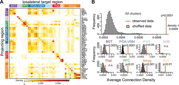
Anatomical connectivity in brain regions associated with pairing.
(A) This heatmap shows normalized connection densities (Knox et al., 2019) from projecting to ipsilateral target regions of interest (ROIs) in the mouse brain. These ROIs are the same as, or larger divisions that contain, the ROIs found to be associated with pair-bond development in our analysis. (B) The top histogram shows results of a permutation test to assess whether hierarchical clusters of chosen ROIs (n = 68 from 189 vole brain samples) in our analysis mirror underlying anatomical connections. Observed connectivity reflects the overall average of cluster means, which is compared to averages from 10,000 iterations of shuffled data (i.e., target regions shuffled for each projecting region). The bottom histograms show the results of permutation tests for mean connectivity within each ROI cluster. Cluster group labels include ‘BST’ (bed nucleus of the stria terminalus) in dark purple, ‘AOB’ (accessory olfactory bulb) in light purple, ‘PFC’ (prefrontal cortex) in green, ‘POA-VMH’ (preoptic area, ventromedial hypothalamus) in dark blue, ‘PVH’ (paraventricular hypothalamus) in light blue, ‘Thal’ (thalamus) in red, ’Aud’ (auditory cortex) in light orange, and ‘Amyg’ (amygdala) in dark orange. Full ROI names are listed in Supplementary file 4.
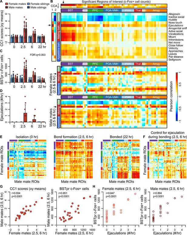
Bed nucleus of the stria terminalis (BST) emerges as a central hub in the bonding network that is associated with mating success in both sexes.
(A) The first dimension of canonical correlation (CC) scores is compared across experiment groups (mean ± standard deviation [SD], n = 11-12 animals/group). (B) Heatmaps represent correlation coefficients among CC scores, region of interest (ROI) c-Fos+ cell counts, and behavior measures. The full dataset is on top (n = 189 animals for correlations involving ultrasonic vocalizations [USVs], n = 187 for all other behaviors), and the bottom two correlograms are for female (n = 23) and male (n = 24) mates. In (B, E, F), warm and cool colors represent positive and negative coefficients, respectively. Arrows mark the ROI (principle nucleus of the BST [BSTpr]) and behavior (ejaculation) with the strongest correlations to CC1. (C) BSTpr activation is compared across groups (n = 11-12 animals/group) with a GLM comparison (ANOVA) followed by a permutation test (10,000 permutations) and false discovery rate (FDR) correction for multiple tests across ROIs. (D) Successful mating events are shown across timepoints (mean ± SD, n = 22-24 dyads/group). (E) Similarity (i.e., Pearson correlation) of bonding network activation is shown in female–male pairs at the 0 hr (n = 11), 2.5 and 6 hr (n = 23) and 22 hr (n = 12) timepoints. (F) Similarity in bonding network activation is shown in female–male pairs (n = 23), using partial Pearson correlations to control for ejaculation rates. (G) Female–male pair similarity is shown for CC1 scores (n = 24 pairs) and BSTpr activation (n = 23 pairs) during bond formation. (H) Pearson correlations are used to associate ejaculation rates with BSTpr activation for female mates (n = 23) and male mates (n = 24). In (A, C, D), mate pairs are in red and sibling pairs in blue (females in lighter hues, males in darker hues). In (B, E, F), cluster group labels include ‘BST’ (bed nucleus of the stria terminalus) in dark purple, ‘AOB’ (accessory olfactory bulb) in light purple, ‘PFC’ (prefrontal cortex) in green, ‘POA-VMH’ (preoptic area, ventromedial hypothalamus) in dark blue, ‘PVH’ (paraventricular hypothalamus) in light blue, ‘Thal’ (thalamus) in red, ’Aud’ (auditory cortex) in light orange, and ‘Amyg’ (amygdala) in dark orange. ROI names and order correspond to Figure 3C. Full ROI names are listed in Supplementary file 4.
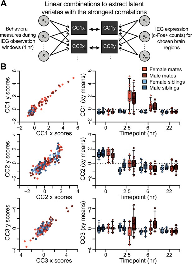
Dimensions of cross-covariance in immediate early gene expression and social behavior.
(A) A schematic of the canonical correlation analysis (CCA) method is shown, where two sets of variables (x and y) are combined linearly to extract latent variates with the strongest correlations (CC1 stronger than CC2, and so on). This analysis outputs x and y scores for each latent variate for each animal subject. In this dataset, x scores represent linear combinations of behavioral measures, and y scores represent linear combinations of region of interest (ROI) c-Fos+ cell counts. (B) On the left, the relationship between x and y scores is shown for all study animals for the first three variates (n = 191 animals). On the right, the means of x and y scores for the first three variates are compared across partner type, sex, and timepoint (n = 11-12 animals/group; boxplots = median, 25–75% quartile, and 95% confidence intervals). Mate pairs are in red and sibling pairs in blue (females in lighter hues, males in darker hues).
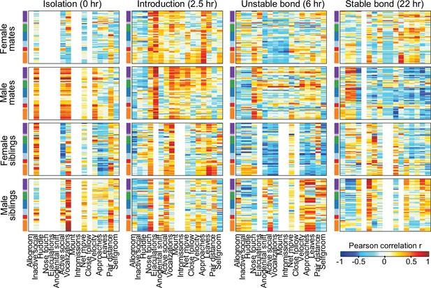
Intra-pair similarity in immediate early gene expression in pairing-associated brain regions.
Heatmaps represent Pearson correlation coefficients, with brain regions on the y-axis (grouped into hierarchical clusters, see Figure 3 for region of interest [ROI] and cluster labels) and behavioral outcomes (during 1 hr observation windows) on the x-axis. Correlation heatmaps are split by partner type, sex, and timepoint (n = 11-12 animals/group). Warm and cool colors indicate positive and negative correlation coefficients, respectively. White indicates behaviors with no variation, meaning that coefficients were not computed (e.g., siblings did not exhibit mating behaviors). ROIs are grouped by hierarchical clusters (see Figure 3). Cluster group labels include ‘BST’ (bed nucleus of the stria terminalus) in dark purple, ‘AOB’ (accessory olfactory bulb) in light purple, ‘PFC’ (prefrontal cortex) in green, ‘POA-VMH’ (preoptic area, ventromedial hypothalamus) in dark blue, ‘PVH’ (paraventricular hypothalamus) in light blue, ‘Thal’ (thalamus) in red, ’Aud’ (auditory cortex) in light orange, and ‘Amyg’ (amygdala) in dark orange. ROI names and order correspond to Figure 3C. Full ROI names are listed in Supplementary file 4.
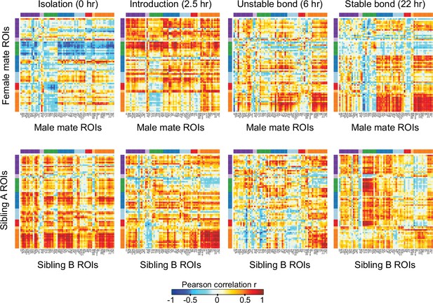
Patterns of association between immediate early gene expression and behavior.
On the top, heatmaps represent Pearson correlation coefficients between selected brain regions of interest (ROIs) in mating pairs (n = 11-12 pairs/timepoint), with female data on the y-axis and male data on the x-axis. On the bottom, heatmaps represent Pearson correlation coefficients between selected ROIs in sibling dyads (n = 11-12 dyads/timepoint), where sibling A data are from animals placed in the left side of chamber during acclimation, and sibling B data are from animals placed on the right side. ROIs are grouped by hierarchical clusters (see Figure 3). Warm and cool colors indicate positive and negative correlation coefficients, respectively. Cluster group labels include ‘BST’ (bed nucleus of the stria terminalus) in dark purple, ‘AOB’ (accessory olfactory bulb) in light purple, ‘PFC’ (prefrontal cortex) in green, ‘POA-VMH’ (preoptic area, ventromedial hypothalamus) in dark blue, ‘PVH’ (paraventricular hypothalamus) in light blue, ‘Thal’ (thalamus) in red, ’Aud’ (auditory cortex) in light orange, and ‘Amyg’ (amygdala) in dark orange. ROI names and order correspond to Figure 3C. Full ROI names are listed in Supplementary file 4.

Working model for neural systems that shape stages of pair-bond development.
(A) A schematic is shown of the network of regions identified in our study, overlaid with regions involved in rodent mating behavior (Pfaus and Heeb, 1997; Veening et al., 2014; Veening and Coolen, 2014). This network is proposed to be involved during the early stages of bond formation (e.g., 2.5 hr timepoint). (B) A schematic is shown of the network of regions identified in our study, overlaid with regions involved in prairie vole pair-bonding behavior (Walum and Young, 2018; Young et al., 2011). This network is proposed to be involved with the middle stages of bond formation when animals are engaged in prolonged mating and affiliative interactions (e.g., 6 hr timepoint). (C) A schematic is shown of the network of regions that are correlated between female and male mates at the 22 hr timepoint in this study. These regions are identified from pairs of regions in which both sexes show high inter-individual similarity (Pearson correlation, r > 0.75). This network is proposed to be involved with the recognition and convergence of behavioral state in bonding partners. The network schematics in (A–C) are adapted from the multi-dimensional scaling of correlations between region activity (Figure 3D). Light gray points represent regions not included in the proposed network. Line thickness and darkness between colored regions represent Pearson correlation r values between the connected regions. Cluster group labels include ‘BST’ (bed nucleus of the stria terminalus) in dark purple, ‘AOB’ (accessory olfactory bulb) in light purple, ‘PFC’ (prefrontal cortex) in green, ‘POA-VMH’ (preoptic area, ventromedial hypothalamus) in dark blue, ‘PVH’ (paraventricular hypothalamus) in light blue, ‘Thal’ (thalamus) in red, ’Aud’ (auditory cortex) in light orange, and ‘Amyg’ (amygdala) in dark orange. Full ROI names are listed in Supplementary file 4.
Videos
Prairie vole reference brain.
The prairie vole reference brain from light-sheet fluorescence microscopy (LSFM) imaging is shown for coronal cross-sections (rostral to caudal) and in a 3D view. Then, coronal cross-sections are shown for the prairie vole atlas (left) alongside whole-brain staining for somatostatin (SST, middle) and fluorescent Nissl (NeuroTrace, right).
Patterns of whole-brain immediate early gene expression during pairing.
First, coronal cross-sections of immediate early gene (IEG) expression are shown for female (first video) and male (second video) prairie voles across all experiment groups split by partner type (mates – top, siblings – bottom) and timepoint (0, 2.5, 6, and 22 hr from left to right, n = 11-12 animals/group). Brightness corresponds to mean voxel c-Fos+ cell counts. These videos are associated with Figure 3—figure supplement 1 (see this figure for the color key). The induction patterns are overlaid with prairie vole atlas boundaries. Next, coronal cross-sections are shown with the results of generalized linear model (GLM) comparisons to identify brain areas associated with bonding (n = 189 vole brain samples). This video is associated with Figure 3A (see this panel for the color key). The reference is overlaid with colored voxels that represent differences between hypothesized (includes partner type effect) and null (no partner type) GLMs. Analysis of variance (ANOVA) tests were used to compare GLMs, with a false discovery rate (FDR) correction across voxels (alpha threshold of q = 0.1). Warm colors indicate voxels with higher c-Fos+ cell counts in mate pairs (GLM test statistic for partner type > 0), and cooler colors indicate voxels with higher c-Fos+ cell counts in siblings (GLM test statistic for partner type < 0). Finally, coronal cross-sections are shown with the results of GLM comparisons to identify brain areas associated with sex differences. The reference is overlaid with colored voxels that represent differences between hypothesized (includes partner type x sex interaction) and null (no partner type x sex interaction) GLMs (ANOVA with FDR q < 0.1). Colored voxels indicate regions where there was an interaction effect, with warm colors indicating a positive interaction term and cool colors indicating a negative interaction term (see Figure 3A color key).
Additional files
-
Supplementary file 1
Statistical comparisons of absolute and relative brain area volumes between prairie voles and mice.
Absolute and relative area volumes (normalized to total brain volume) are compared between prairie voles (n = 190 voles, 94 males and 96 females) and male mice (n = 108) with negative binomial regression models. Absolute brain area volumes are all statistically significant bigger in the prairie vole compared to the mouse, but none the ratios of area volume (relative to the whole brain) were statistically different between species. Mean, standard deviation (SD), p-values, and false discovery rate (FDR) correction of the p-values are presented for each region.
- https://cdn.elifesciences.org/articles/87029/elife-87029-supp1-v2.xlsx
-
Supplementary file 2
Statistical comparisons of absolute and relative brain area volumes between male and female prairie voles.
Absolute and relative area volumes (normalized to total brain volume) are compared between 94 male and 96 female prairie voles with negative binomial regression models. No statistical differences were found in these sex comparisons. Mean, standard deviation (SD), p-values, and false discovery rate (FDR) correction of the p-values are presented for each region.
- https://cdn.elifesciences.org/articles/87029/elife-87029-supp2-v2.xlsx
-
Supplementary file 3
Prairie vole behavior ethogram.
Descriptions are included for automated, semi-automated, and manually scored behavioral measures.
- https://cdn.elifesciences.org/articles/87029/elife-87029-supp3-v2.xlsx
-
Supplementary file 4
Statistical results from comparisons of generalized linear models across brain regions.
Null generalized linear models (GLMs) and hypothesized (i.e., ‘bonding’) GLMs were compared with analysis of variance (ANOVA) tests for each region of interest (ROI, 824 regions, n = 189 brain samples, 11-12 samples/group). The ANOVA F-statistics are reported alongside p-values computed from permutation tests (10,000 shuffles). The corresponding q-values were computed with the false discovery rate (FDR) method to correct for multiple tests.
- https://cdn.elifesciences.org/articles/87029/elife-87029-supp4-v2.xlsx
-
MDAR checklist
- https://cdn.elifesciences.org/articles/87029/elife-87029-mdarchecklist1-v2.docx


