Research Article

Neuroscience

Firing rate adaptation affords place cell theta sweeps, phase precession, and procession

School of Psychological and Cognitive Sciences, IDG/McGovern Institute for Brain Research, Center of Quantitative Biology, Peking-Tsinghua Center for Life Sciences, Academy for Advanced Interdisciplinary Studies, Peking University, China
Institute of Cognitive Neuroscience, University College London, United Kingdom
Department of Psychology, Tsinghua University, China
Lyda Hill Department of Bioinformatics, O’Donnell Brain Institute, The University of Texas Southwestern Medical Center, United States
School of Computer Science, Peking University, China
Department of Neuroscience, Physiology and Pharmacology, University College London, United Kingdom

Jul 22, 2024

https://doi.org/10.7554/eLife.87055.4

Open access
Copyright information

Version of Record: July 22, 2024 Read the peer reviews
Reviewed Preprint: v3 June 5, 2024
Reviewed Preprint: v2 January 11, 2024
Reviewed Preprint: v1 May 17, 2023

Download
A two-part list of links to download the article, or parts of the article, in various formats.
Downloads (link to download the article as PDF)
- Article PDF
Open citations (links to open the citations from this article in various online reference manager services)
- Mendeley
Cite this article (links to download the citations from this article in formats compatible with various reference manager tools)
Tianhao Chu

Zilong Ji

Junfeng Zuo

Yuanyuan Mi

Wen-hao Zhang

Tiejun Huang

Daniel Bush

Neil Burgess

Si Wu

(2024)
Firing rate adaptation affords place cell theta sweeps, phase precession, and procession

eLife 12:RP87055.

https://doi.org/10.7554/eLife.87055.4
- Download BibTeX
- Download .RIS
Cite
Share
CommentOpen annotations (there are currently 0 annotations on this page).

Figures
Videos
Tables
Additional files

16 figures, 4 videos, 3 tables and 2 additional files

Figures

Figure 1

Download asset Open asset

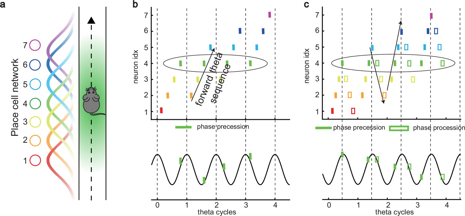
Theta sequence and theta phase shift of place cell firing.

(a) An illustration of an animal running on a linear track. A group of place cells each represented by a different color are aligned according to their firing fields on the linear track. (b) An …

Figure 2

Download asset Open asset

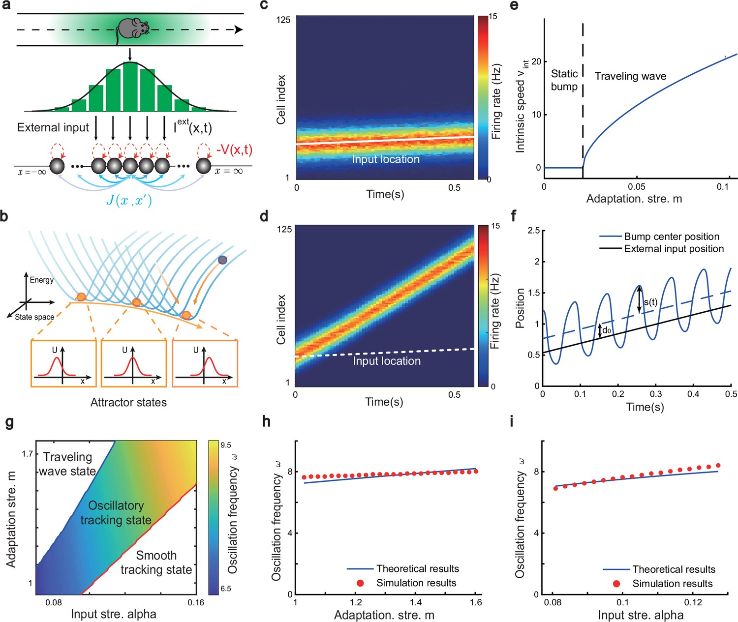
The network architecture and tracking dynamics.

(a) A one-dimensional (1D) continuous attractor neural network (CANN) formed by place cells. Neurons are aligned according to the locations of their firing fields on the linear track. The recurrent …

Figure 3

Download asset Open asset

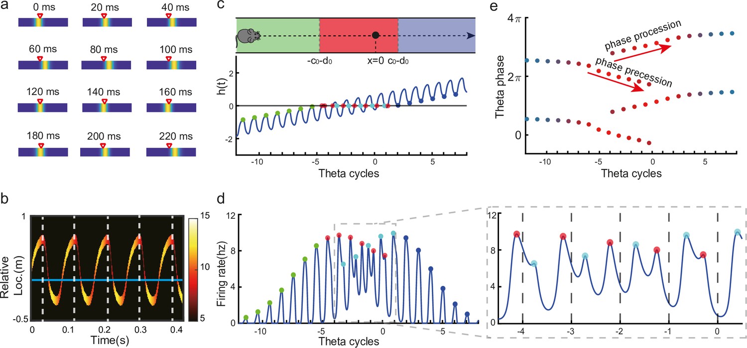
Oscillatory tracking accounts for theta sweeps and theta phase shift.

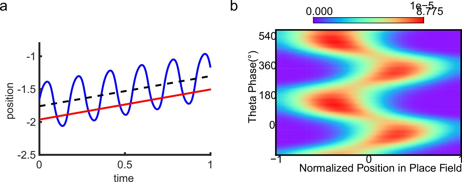
(a) Snapshots of the bump oscillation along the linear track in one theta cycle (0–140 ms). Red triangles indicate the location of the external moving input. (b) Decoded relative positions based on …

Figure 4

Download asset Open asset

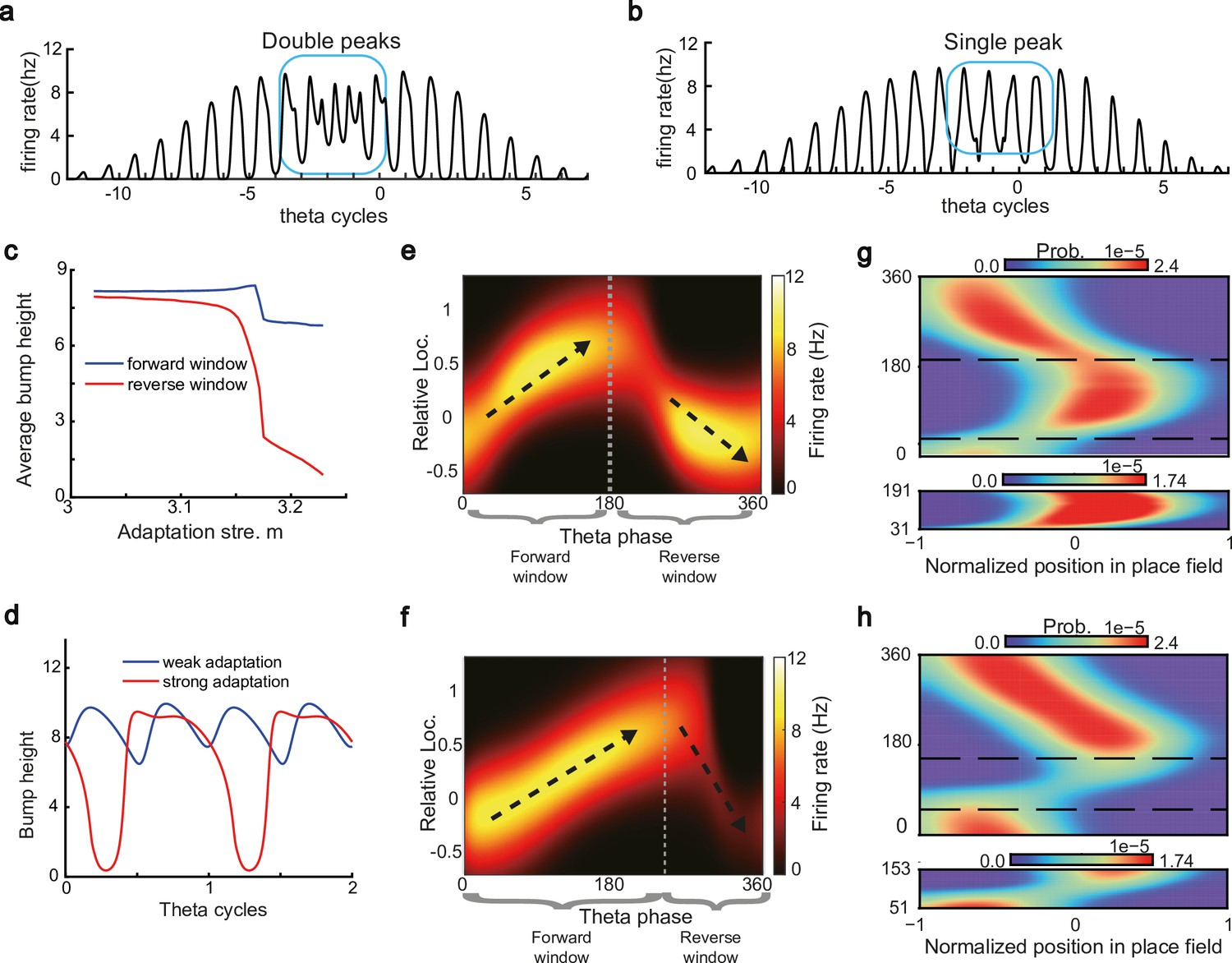
Different adaptation strengths account for the emergence of bimodal and unimodal cells.

(a) The firing rate trace of a typical bimodal cell in our model. Blue boxes mark the phase shift stage. Note that there are two peaks in each theta cycle. (b) The firing rate trace of a typical …

Figure 5

Download asset Open asset

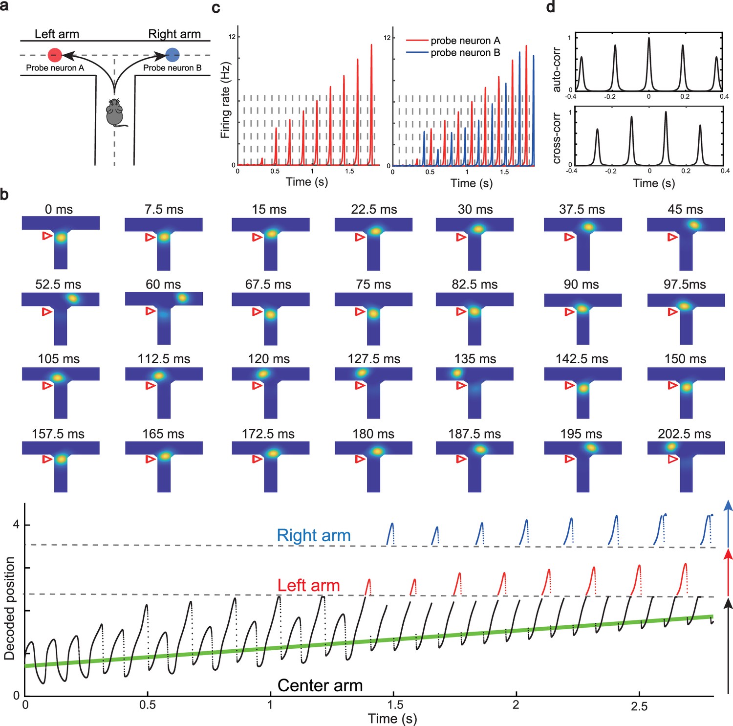
Constant cycling of future positions in a T-maze environment.

(a) An illustration of an animal navigating a T-maze environment with two possible upcoming choices (the left and right arms). (b) Upper panel: Snapshots of constant cycling of theta sweeps on two …

Figure 6

Download asset Open asset

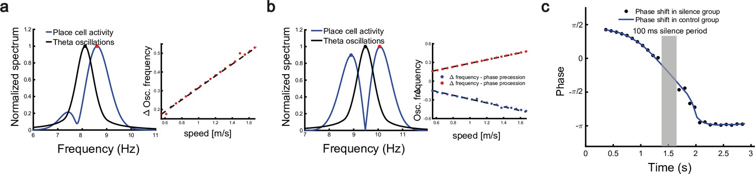
Robust phase coding of position.

(a) Left: normalized spectrum of bump oscillation (black curve) and the oscillation of a unimodal cell (blue curve). Right: linear relationship between the frequency difference and the running …

Appendix 1—figure 1

Download asset Open asset

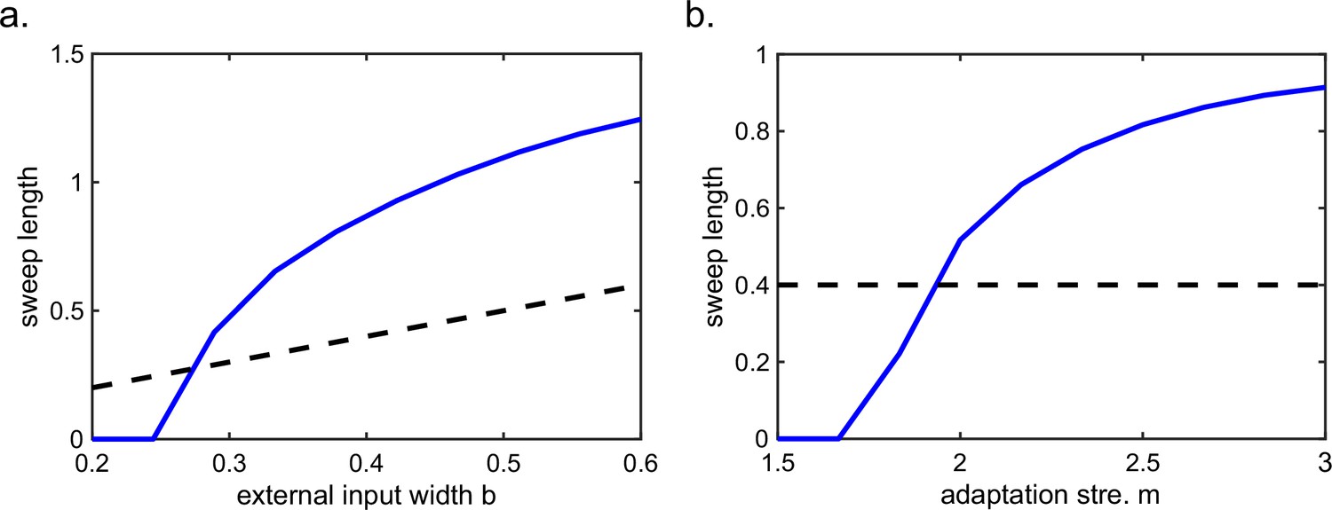
Sweep length is not bounded by the external input width.

(a) The sweep length is positively but not linearly related with the external input width. (b) With fixed external input width, increasing the adaptation strength the sweep length can exceed the …

Appendix 1—figure 2

Download asset Open asset

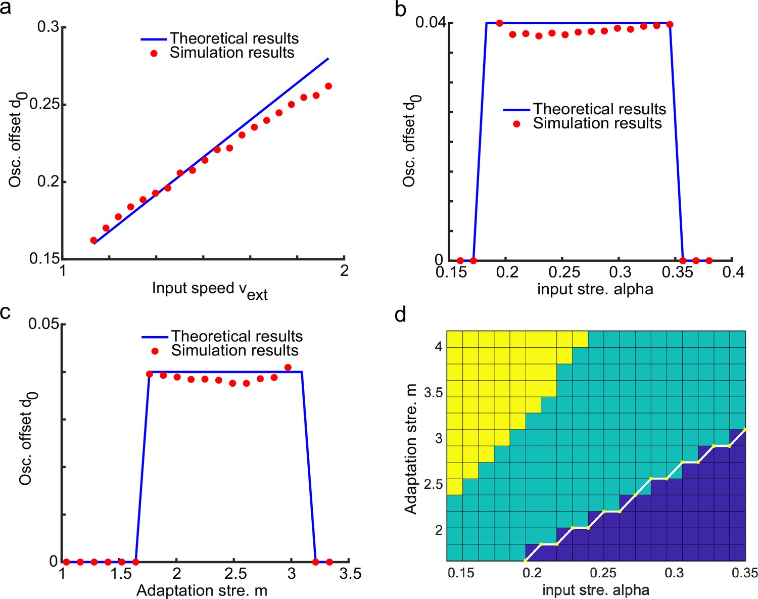
Verifying theoretical results with numerical simulations.

(**a–c**) Simulation results of the average offset $d_{0}$ as a function of $v_{e x t}$ , $α$ , and $m$ , respectively. (d) The phase diagram of network states. The yellow area represents the traveling wave state, the …

Appendix 1—figure 3

Download asset Open asset

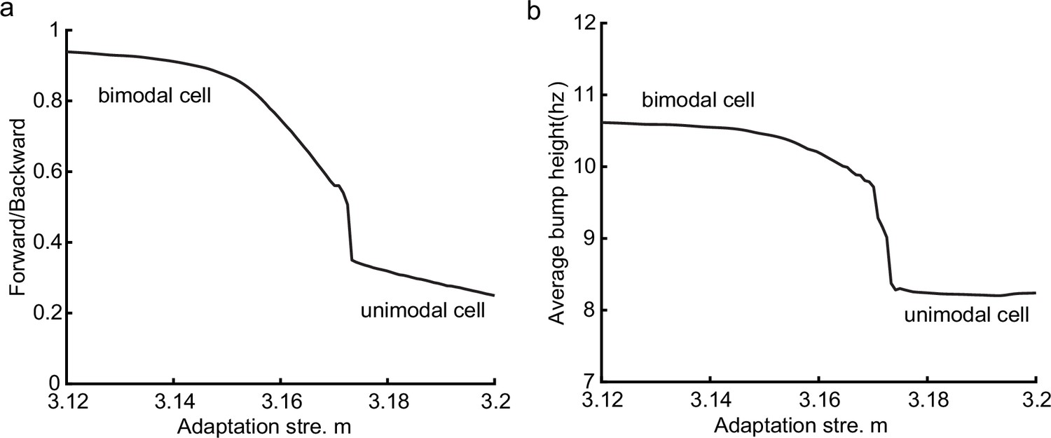
Activity bump height as a function of the adaptation strength.

(a) The ratio between the average bump height during forward window and the average bump height during backward window as function of the adaptation $m$ . When the adaptation strength is relatively …

Appendix 1—figure 4

Download asset Open asset

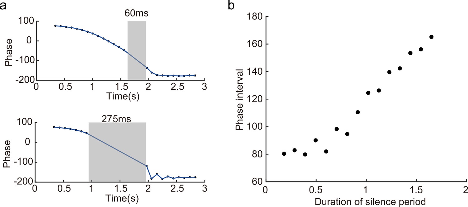
Persistent phase shift with variable silencing periods.

(a) Two examples of the persisting phase shift after transient silencing. Upper panel: The silencing duration is 60 ms. Upper panel: The silencing duration is 275 ms. (b) The phase interval before …

Appendix 1—figure 5

Download asset Open asset

Persistent bimodal phase shift after transient silencing.

The parameters are: $α = 0.19$ , $m = 3.03$ , $a = 0.4$ , $k = 5$ , $J_{0} = 1$ , $N = 512$ , $τ = 3 m s$ , $τ_{v} = 144 m s$ , $ρ = 20.37$ , $v_{e x t} = 0.3 m / s$ . This figure relates to Figure 6 in the main text.

Appendix 1—figure 6

Download asset Open asset

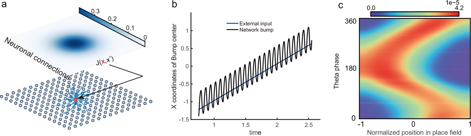
Theta sweeps and theta phase shift in a two-dimensional (2D) continuous attractor neural network (CANN).

(a) A demonstration of the 2D CANN. (b) The trajectory of the bump center and external input center when the input is moving along the x-axis in the 2D CANN. (c) Theta phase as a function of the …

Appendix 1—figure 7

Download asset Open asset

Theta oscillation of the population activities during the theta sweep state.

This figure relates to Figure 4 in the main text.

Appendix 1—figure 8

Download asset Open asset

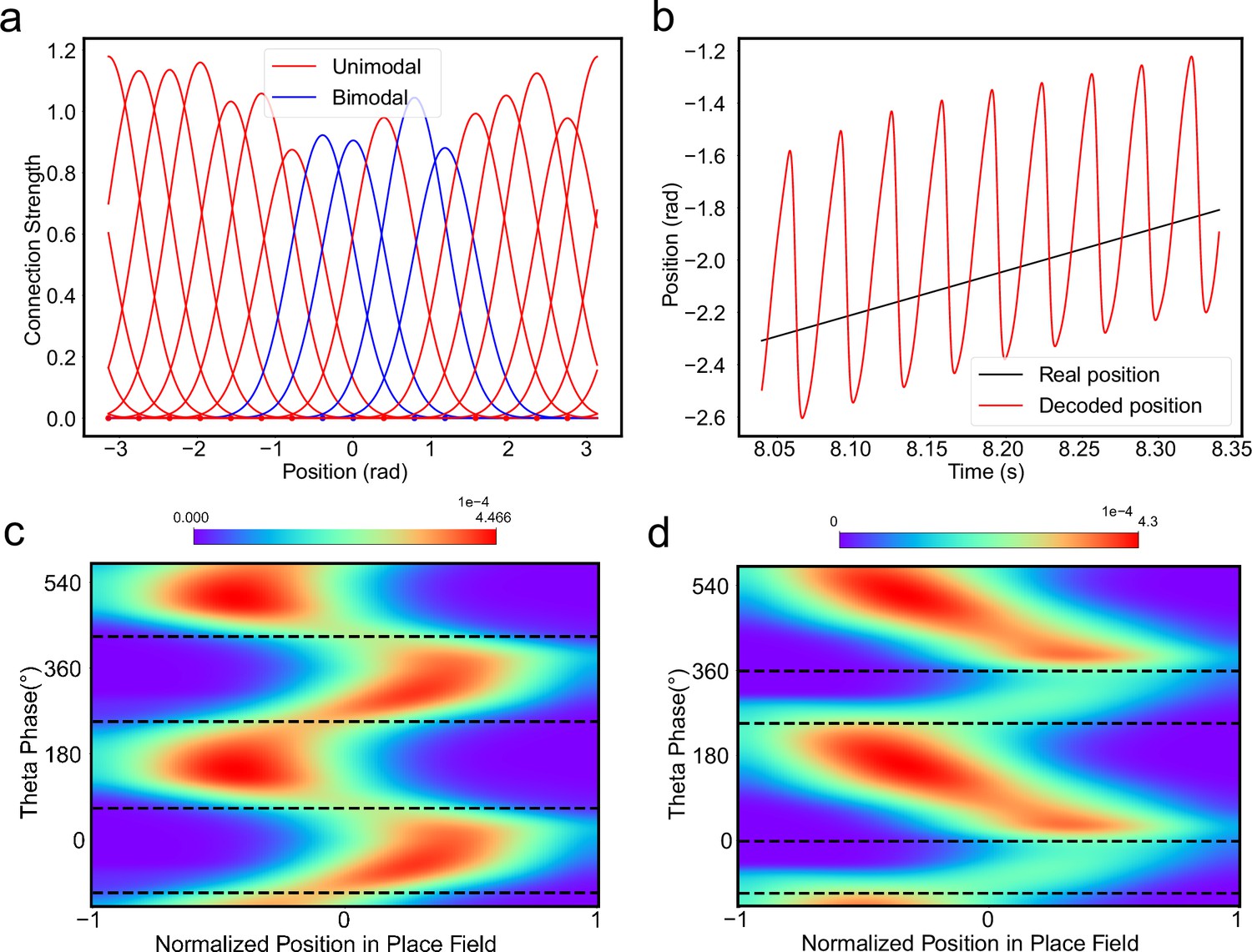
A-continuous attractor neural network (CANN) with heterogeneous connection strength generate oscillatory tracking to account for theta phase shift.

(a) The synaptic connection strength profile of the neurons in the network. The blue lines represent the synaptic strengths of the neurons which turn out to be bimodal neurons, while the red lines …

Appendix 1—figure 9

Download asset Open asset

Oscillatory tracking behavior accounts for theta phase shift with $τ = 10 m s$ .

(a) Oscillatory tracking behavior. (b) Bimodal phase shift of one example neuron. $τ = 10 m s, τ_{v} = 480 m s, α = 0.3, m = 6$ , Other parameters are set equal with the Figure 2 in the main text. This figure relates to Figure 2 in the main …

Appendix 1—figure 10

Download asset Open asset

Spatiotemporal tracking dynamics when the adaptation strength is low (start from 0).

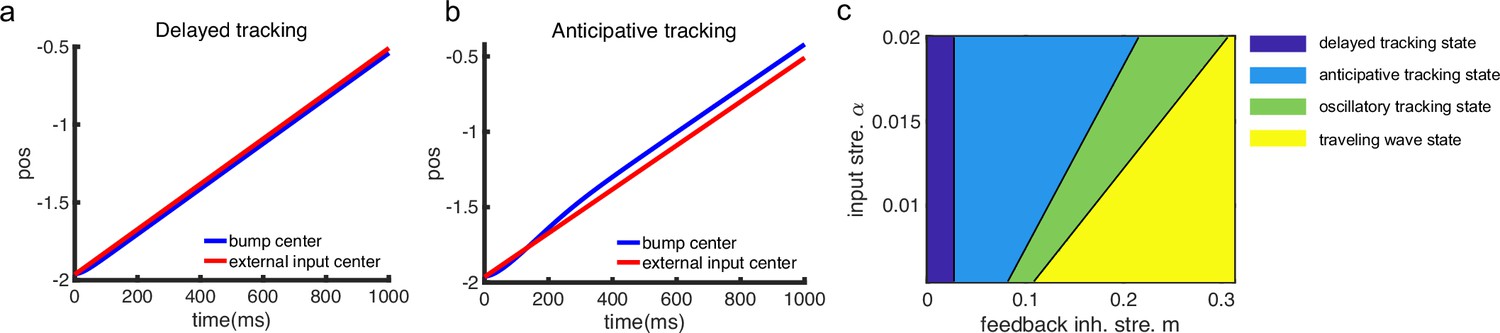
(a) The tracking behavior when the adaptation strength $m = 0$ ( $α = 0.02$ ). The network bump can generate a bump to track the external input stimuli smoothly but with a constant lagging distance which is …

Videos

Video 1

Download asset

posterframe for video — The title of this video is: Three dynamical states of Adaptive Continous Attractor Neural Network.

Video 2

Download asset

Video 3

Download asset

Video 4

Download asset

Tables

Appendix 1—table 1

Commonly used parameter values in the simulation of the linear track environment.

Parameters	Values
Number of place cells: $N$	512
Time constant of neural firing: $τ$	3 ms
Time constant of spike frequency adaptation: $τ_{v}$	144 ms
Neuron density: $ρ$	$256 / π$
Recurrent connection range (Gaussian width): $a$	0.4 m
Width of external input (Gaussian width): $σ$	0.4 m
Recurrent connection strength: $J_{0}$	0.2
Gain factor: $g$	5
Global inhibition strength: $k$	5
Moving speed of the external input: $v_{e x t}$ (m/s)	1.5
Time interval: $δ t$	0.3 s
Simulation duration: $T$	10 s

Appendix 1—table 2

Figure-specific parameter values for input strength $α$ and adaptation strength $m$ .

Figures/parameters	$α$	$m$
An example of smooth tracking (Appendix 1—figure 2c)	0.19	0
An example of traveling wave (Appendix 1—figure 2d)	0	0.31
Intrinsic speed vs. adaptation strength (Appendix 1—figure 2e)	0	0:0.05:0.1
Phase diagram (Appendix 1—figure 2g)	0.05:0.001:0.16	0.9:0.01:1.8
Oscillatory tracking (bimodal) (Appendix 1—figure 4a, e, g)	0.19	3.02
Oscillatory tracking (unimodal) (Appendix 1—figure 4b, f, h)	0.19	3.125

Appendix 1—table 3

Parameters values in the simulation of the T-maze environment.

Parameters	Values
Number of cells central/left/right: $N_{1}, N_{2}, N_{3}$	3000/1500/1500
Time constant of neural firing: $τ$	3 ms
Time constant of spike frequency adaptation: $τ_{v}$	144 ms
Neuron density: $ρ$	${(128 / π)}^{2}$
Recurrent connection range (Gaussian width): $a$	0.3
Recurrent connection strength: $J_{0}$	1.25 ∗ 10^-2
Gain factor: $g$	20
Global inhibition strength: $k$	1.25
Moving speed of the external input: $v_{e x t}$ (m/s)	1.5
Input strength: $α$	2
Adaptation strength: $m$	3.96
Time interval: $δ t$	0.3 s
Simulation duration: $T$	3.3 s

Additional files

MDAR checklist: https://cdn.elifesciences.org/articles/87055/elife-87055-mdarchecklist1-v1.docx
Download elife-87055-mdarchecklist1-v1.docx
Source code 1 Modelling code for ‘Firing rate adaptation affords place cell theta sweeps, phase precession, and procession’.: https://cdn.elifesciences.org/articles/87055/elife-87055-code1-v1.zip
Download elife-87055-code1-v1.zip

Downloads (link to download the article as PDF)

Open citations (links to open the citations from this article in various online reference manager services)

Cite this article (links to download the citations from this article in formats compatible with various reference manager tools)

Figures

Theta sequence and theta phase shift of place cell firing.

The network architecture and tracking dynamics.

Oscillatory tracking accounts for theta sweeps and theta phase shift.

Different adaptation strengths account for the emergence of bimodal and unimodal cells.

Constant cycling of future positions in a T-maze environment.

Robust phase coding of position.

Sweep length is not bounded by the external input width.

Verifying theoretical results with numerical simulations.

Activity bump height as a function of the adaptation strength.

Persistent phase shift with variable silencing periods.

Persistent bimodal phase shift after transient silencing.

Theta sweeps and theta phase shift in a two-dimensional (2D) continuous attractor neural network (CANN).

Theta oscillation of the population activities during the theta sweep state.

A-continuous attractor neural network (CANN) with heterogeneous connection strength generate oscillatory tracking to account for theta phase shift.

Oscillatory tracking behavior accounts for theta phase shift with $τ = 10 m s$ .

Spatiotemporal tracking dynamics when the adaptation strength is low (start from 0).

Videos

The title of this video is: Three dynamical states of Adaptive Continous Attractor Neural Network.

The title of this video is: Neuronal activities during bi-directional oscillatory tracking state.

The title of this video is: Neuronal activities during uni-directional oscillatory tracking state.

The title of this video is: Bump oscillation in T-maze environment.

Tables

Commonly used parameter values in the simulation of the linear track environment.

Figure-specific parameter values for input strength $α$ and adaptation strength $m$ .

Parameters values in the simulation of the T-maze environment.

Additional files

MDAR checklist

Source code 1

Download links

Be the first to read new articles from eLife

Share this article

Cite this article

Theta sequence and theta phase shift of place cell firing.

The network architecture and tracking dynamics.

Oscillatory tracking accounts for theta sweeps and theta phase shift.

Different adaptation strengths account for the emergence of bimodal and unimodal cells.

Constant cycling of future positions in a T-maze environment.

Robust phase coding of position.

Sweep length is not bounded by the external input width.

Verifying theoretical results with numerical simulations.

Activity bump height as a function of the adaptation strength.

Persistent phase shift with variable silencing periods.

Persistent bimodal phase shift after transient silencing.

Theta sweeps and theta phase shift in a two-dimensional (2D) continuous attractor neural network (CANN).

Theta oscillation of the population activities during the theta sweep state.

A-continuous attractor neural network (CANN) with heterogeneous connection strength generate oscillatory tracking to account for theta phase shift.

Spatiotemporal tracking dynamics when the adaptation strength is low (start from 0).

The title of this video is: Three dynamical states of Adaptive Continous Attractor Neural Network.

The title of this video is: Neuronal activities during bi-directional oscillatory tracking state.

The title of this video is: Neuronal activities during uni-directional oscillatory tracking state.

The title of this video is: Bump oscillation in T-maze environment.

Commonly used parameter values in the simulation of the linear track environment.

Figure-specific parameter values for input strength α<math id="inf446"><semantics><mi>α</mi></semantics></math> and adaptation strength m<math id="inf447"><semantics><mi>m</mi></semantics></math>.

Parameters values in the simulation of the T-maze environment.

MDAR checklist

Source code 1

Figure-specific parameter values for input strength $α$ and adaptation strength $m$ .