Generating variability from motor primitives during infant locomotor development
Figures
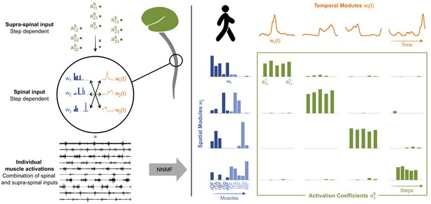
Theory of modularity and modular organization of adult walking.
Left: the theory of modularity postulates that individual muscle activations result from the combination of basic spinal structures called locomotor primitives, which are of two types: spatial (blue) and temporal (orange) modules. According to the space-by-time model that is used here, the brain activates those modules through a supraspinal input (green) that specifies which amplitude of activation has to be allocated to each possible pair of spatial and temporal modules. In humans, non-negative matrix factorization (NNMF) is used to identify the underlying motor primitives and their activation coefficients from electromyographic (EMG) data. Right: illustration of NNMF applied to five right steps of walking in a human adult. EMG patterns can be decomposed into four spatial modules (blue) and four temporal modules (orange). Muscles from both sides can be allocated to a same spatial module to form bilateral modules. Within each spatial module, weightings are plotted for muscles m1 to m10 in the following order: rectus femoris, tibialis anterior, biceps femoris, soleus, and gluteus medius (right muscles in dark blue followed by left muscles in light blue). Activation coefficients (green) represent the level of activation of each possible pair of spatial and temporal modules during five steps. Two features are typical of adults’ modular organization: the stability of activation (activations coefficients remain stable during the five steps) and the selectivity of activation (one spatial module is always activated with only one temporal module and vice versa).
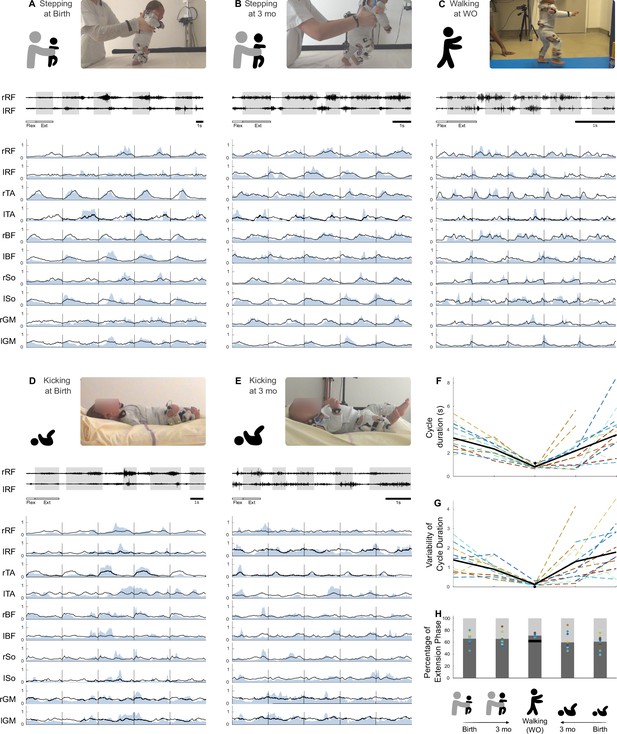
Development of basic electromyographic (EMG) and kinematic parameters.
(A–E) Example of EMG data for each age and behavior in one infant. A set of five cycles of flexion and extension is presented for each age and behavior. High-pass-filtered data are shown for two muscles (extension phases appear on a gray background). The 10 muscles are then pictured as completely preprocessed (i.e. filtered and normalized in amplitude and time, blue envelope). The black line is the averaged signal across the five pictured cycles. The scale of 1 s is displayed at the bottom of each figure. RF, rectus femoris; TA, tibialis anterior; BF, biceps femoris; So, soleus; GM, gluteus medius. (F–I) Evolution of several features starting from birth to walking onset for stepping or kicking. Individual data are shown in dotted line with the same color code as in Figure 3. Each point was computed as a mean score for each individual (see section ‘Number of cycles included in the analysis’). The black bold line represents the averaged values across individuals. The black point (or trait in F) represents the adult landmark. (F) Cycle duration. (G). Kinematic variability (standard deviation of cycle duration divided by averaged cycle duration). (H) Proportion of flexion and extension phases.
-
Figure 2—source data 1
Individual data regarding basic electromyographic (EMG) and kinematic parameters (corresponding to Figure 2F–H).
- https://cdn.elifesciences.org/articles/87463/elife-87463-fig2-data1-v1.xlsx
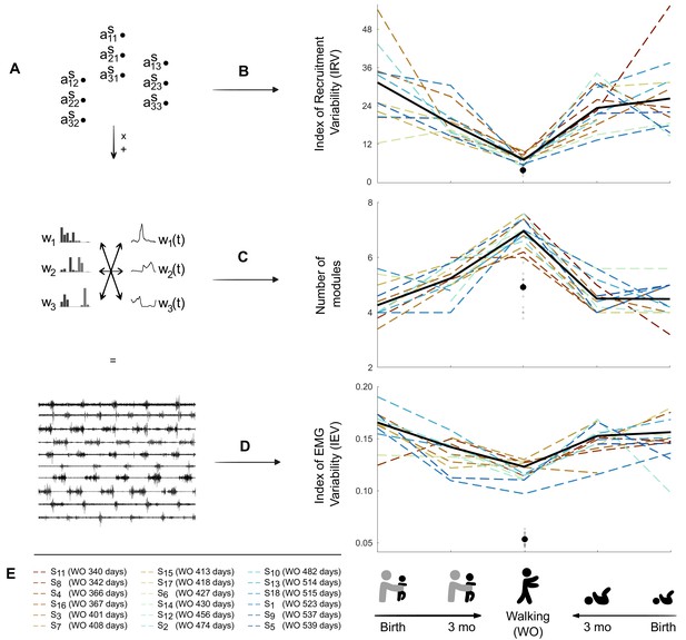
Decrease in variability between birth and walking onset associated with modifications of the underlying set of motor primitives.
(A) Computational elements contributing to the electromyography (EMG) and their trial-to-trial variability (from top do down: activation coefficients, spatial and temporal modules, and muscle outputs). (B–D). Graphs (B–D) show how changes within the upper levels can explain the resulting motor variability during infant locomotor development. Individual data are represented as dotted lines. Each point was computed as a mean score for each individual (see section ‘Number of cycles included in the analysis’). The black bold line represents the averaged values across individuals. The black point indicates the adult landmark, and the gray diamonds indicate individual values from 20 adults (Supplementary file 1c). (B) Variability of module activations, assessed by the index of recruitment variability (IRV). IRV represents the variability of the input that specifies which amplitude of activation has to be allocated to each possible pair of spatial and temporal modules. This index decreases from birth to walking onset considering stepping or kicking as neonatal behavior. (C) Number of spatial and temporal modules, which increases from birth to walking onset considering stepping or kicking as neonatal behavior (D) Index of EMG variability (IEV, same as in Figure 2I). This index decreases from birth to walking onset, considering stepping or kicking as neonatal behavior. (E) Figure legend. Each individual is represented by a color throughout the article. To take into account the variability of walking onset in our representations, colors of each individual are sorted according to their age of walking onset.
-
Figure 3—source data 1
Individual data regarding electromyographic (EMG) output and modeling of the modular organization from birth to walking onset (corresponding to Figure 3B–D).
- https://cdn.elifesciences.org/articles/87463/elife-87463-fig3-data1-v1.xlsx
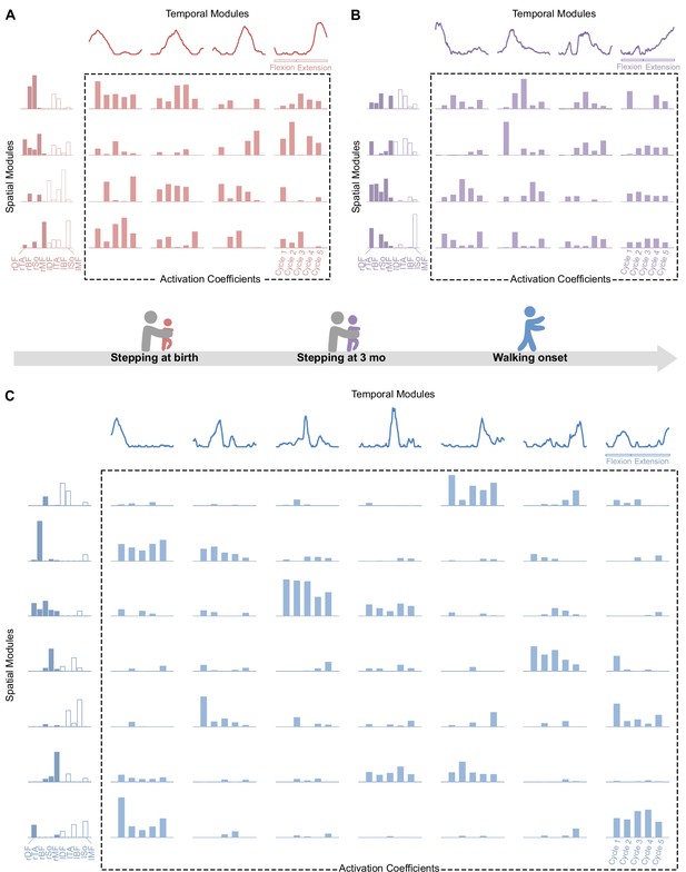
Modular organization at each age in a representative individual.
At each age, electromyographic (EMG) patterns can be decomposed into spatial modules and temporal modules (orange). Within each spatial module, weightings are plotted for muscles m1 to m10 in the following order: rectus femoris, tibialis anterior, biceps femoris, soleus, and gluteus medius (right muscles in dark colors followed by left muscles in light colors). Activation coefficients (at the crossing between each spatial and temporal modules) represent the level of activation of each possible pair of spatial and temporal modules during five steps. (A-B) At birth (red, top left) and 3 mo (purple, top right), EMG activity of stepping can be decomposed into four spatial and four temporal modules. (C) At walking onset (blue, bottom), EMG activity needs to be decomposed into seven spatial and seven temporal modules to get the same quality of modeling than at birth and 3 mo with less modules. Activation coefficients are highly variable at birth and 3 mo and less variable in toddlerhood, with some pairs that are nearly never activated across the five cycles. Note that toddler activations are still more variable than in adults (Figure 1).
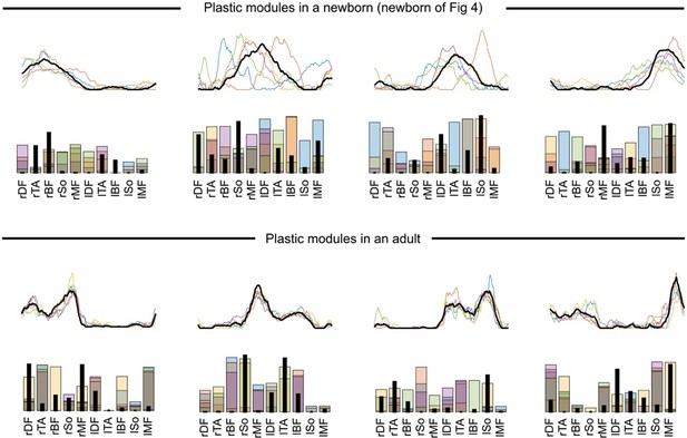
In our analysis, we implicitly assumed that modules cannot vary from cycle to cycle (very short time scale) but that they can vary across development (long time scale).
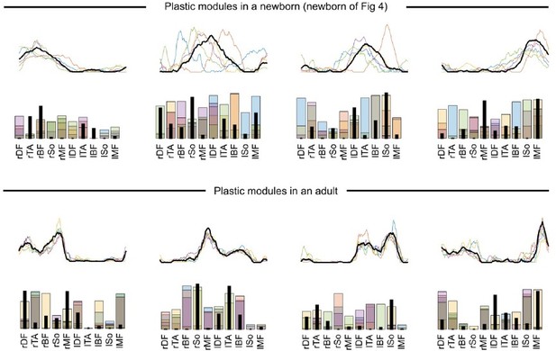
This is the common assumption in muscle synergy analyses (e.g. d’Avella et al., 2003). Nevertheless, to test whether our findings hold if we allow modules to vary across cycles, we reproduced our analysis with the method presented in Cheung et al., 2020a. Here the method was adapted to our space-by-time model by extracting trial-specific w_is(t) and w_js using the global/fixed w_i(t) and w_j as initial estimates of the iterative algorithm. Under this hypothesis, we estimated the short-term plasticity of spatial and temporal modules by computing the sum of point-by-point standard errors across modules from different cycles. This figure illustrates the modules obtained with the plastic-modules approach: the algorithm was initialized with modules that were identified through the original approach and identified different modules for each of the five cycles (results are depicted for a newborn and for an adult individual, with temporal modules on top of spatial modules).
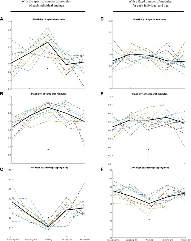
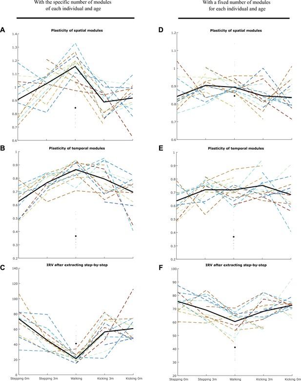
Using the approach presented in Figure 4—figure supplement 1, we computed the plasticity of spatial modules, temporal modules, and activation coefficients (i.e. the IRV, Index of Recruitment Variability) for the specific number of modules of each individual and age (A–C) and for a number of modules fixed to 4 (D–F).
Individual data are shown in dotted line with the same color code as in Figure 3. Each point is computed as a mean score for each individual (see section ‘Number of cycles included in the analysis’). The bold line represents the averaged values across individuals. The black point indicates the adult landmark, and the gray diamonds indicate individual values from 20 adults. In any case, the main effect of the article (decrease of the IRV with age) was persistent, indicating that the algorithm explains better the variability of newborn data by the variability of activation coefficients than for toddlers’ data even under the hypothesis that modules could be plastic in the short-term (i.e. cycle-to-cycle). We repeated this analysis with or without initiating the activation coefficients, and with or without gathering modules by best matching pairs afterward, and found similar results.
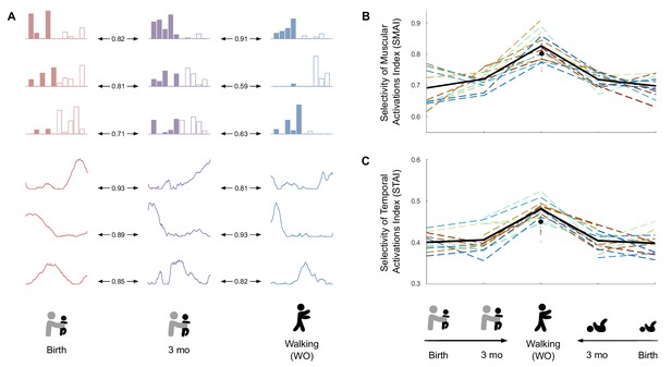
Development of modules’ structure from birth to walking onset.
(A) Similarity of modules between ages in a given individual according to the best matching pair method. (B) Selectivity of muscular activations index (SMAI). (C) Selectivity of temporal activations index (STAI). Both indexes increase between birth and walking onset considering stepping or kicking as neonatal behavior. Individual data are shown in dotted line with the same color code as in Figure 3. Each point is computed as a mean score for each individual (see section ‘Number of cycles included in the analysis’). The bold line represents the averaged values across individuals. The black point indicates the adult landmark, and the gray diamonds indicate individual values from 20 adults (Supplementary file 1c).
-
Figure 5—source data 1
Individual data regarding modules’ structure from birth to walking onset (corresponding to Figure 5B and C).
- https://cdn.elifesciences.org/articles/87463/elife-87463-fig5-data1-v1.xlsx
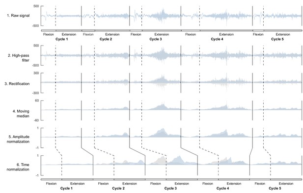
Processing of electromyographic (EMG) data preceding factorization.
Each line shows one step of the preprocessing for an ensemble of five flexion and extension cycles for one muscle. On each graph, the blue signal represents the named step and the gray signal the previous step (i.e. from the above line). This process is applied to raw data before computing the index of EMG variability and before factorizing the signal to identify motor modules.
Videos
Video of participant 5 kicking at 2 days old and 86 days old.
Video of participant 6 stepping at 2 days old and 74 days old, and walking at 434 days old.
Tables
Summary of the role of the main variables of the study.
| Short name | Role |
|---|---|
| Index of EMG variability (IEV) | Represents the cycle-to-cycle variability of EMG data across five alternated cycles of flexion and extension of the lower limb. |
| Variance accounted for (VAF) | Represents the goodness of fit of the model of modularity for a given number of modules. When the VAF for a fixed number of four spatial and temporal modules is computed, it quantifies how well experimental data can be modeled as originating from four modules. |
| Number of modules | Represents the smallest number of invariant spatial and temporal elements in which the EMG signals can be factorized (chosen as the smallest number allowing to reach a VAF > 0.75). |
| Index of recruitment variability (IRV) | Represents the extent to which spatial and temporal modules are steadily (lower value) or variably activated across cycles to produce the EMG outputs (higher value). |
| Index of recruitment selectivity (IRS) | Represents the extent to which spatial modules can be activated with different temporal modules (lower values) or exclusively activated with a given temporal module (higher value). |
| Selectivity of muscular activations index (SMAI) | Represents the extent to which spatial modules each control numerous muscles at a time (lower value) or a few muscles at a time (higher value). |
| Selectivity of temporal activations index (STAI) | Represents the extent to which temporal modules each control muscles during a long time (lower value) or during a shorter peak of time (higher value). |
-
EMG, electromyography.
Summary of individual characteristics.
| Subject ID | Gender | Birth weight (kg) | Birth heigh t (cm) | Age (days) | Precursor that could be observed (T for treadmill, O for overground) | |||
|---|---|---|---|---|---|---|---|---|
| First visit | Second visit | Walking onset | Third visit | |||||
| 1 | F | 3.05 | 48.5 | 21 | 91 | 523 | 535 | Stepping (T) and kicking |
| 2 | M | 4.02 | 52 | 2 | 98 | 474 | 499 | Stepping (T) and kicking |
| 3 | F | 3.71 | 52 | 3 | 87 | 401 | 412 | Stepping (O) and kicking |
| 4 | M | 3.46 | 48 | 2 | 98 | 366 | 371 | Stepping (O) and kicking |
| 5 | F | 3.07 | 50 | 2 | 86 | 539 | Kicking | |
| 6 | M | 3.74 | 51 | 2 | 74 | 427 | 434 | Stepping (O) and kicking |
| 7 | F | 3.68 | 50 | 86 | 408 | 431 | Stepping (T) and kicking | |
| 8 | M | 2.99 | 50 | 2 | 79 | 342 | 365 | Stepping (O) and kicking |
| 9 | M | 2.95 | 48 | 2 | 79 | 537 | 555 | Stepping (T) and kicking |
| 10 | F | 3.46 | 50 | 2 | 582 | 597 | Stepping (T) and kicking | |
| 11 | M | 3.47 | 51 | 1 | 90 | 340 | 409 | Kicking |
| 12 | M | 3.39 | 51 | 2 | 122 | 456 | 478 | Stepping (T) and kicking |
| 13 | M | 3.66 | 49 | 2 | 117 | 514 | 536 | Stepping (O) and kicking |
| 14 | M | 3.28 | 48.5 | 21 | 82 | 430 | 446 | Stepping (O) and kicking |
| 15 | F | 3.89 | 51 | 2 | 116 | 413 | 428 | Stepping (O) and kicking |
| 16 | M | 3.55 | 52 | 2 | 120 | 367 | 380 | Stepping (T) and kicking |
| 17 | M | 3.76 | 51 | 8 | 105 | 418 | Stepping (T) and kicking | |
| 18 | F | 3.50 | 49 | 17 | 101 | 515 | Stepping (O) and kicking | |
Overview of data included in the analysis.
| Participant ID | Overview of data included in the analysis | ||||
|---|---|---|---|---|---|
| Stepping | Walking onset | Kicking | |||
| Birth | 3 months old | 3 months old | Birth | ||
| 1 | 8 | 5 | 8 | 11 | 6 |
| 2 | 5 | 9 | 22 | 5 | |
| 3 | 7 | 5 | 8 | 5 | |
| 4 | 7 | 5 | 8 | 6 | |
| 5 | 12 | 7 | |||
| 6 | 6 | 5 | 7 | 8 | |
| 7 | 16 | 9 | 6 | ||
| 8 | 6 | 6 | 12 | 5 | 5 |
| 9 | 6 | 8 | 22 | 12 | 8 |
| 10 | 6 | 13 | 6 | ||
| 11 | 7 | 5 | 6 | ||
| 12 | 9 | 18 | 10 | 5 | |
| 13 | 5 | 5 | 20 | 6 | 6 |
| 14 | 6 | 5 | 7 | 9 | |
| 15 | 8 | 7 | 8 | ||
| 16 | 15 | 11 | 7 | 8 | 5 |
| 17 | 9 | 13 | 7 | 5 | |
| 18 | 11 | 9 | 8 | 5 | |
| Total number of participants included in the analysis | 11 | 15 | 15 | 15 | 15 |
| Total number of steps included in the analysis | 84 | 122 | 170 | 115 | 95 |
Additional files
-
Supplementary file 1
Detailed statistics and supplementary individual data.
(a) Summary of p-values associated with Wilcoxon tests. p-Values are considered significant for p<0.05 (dark gray) and a trend is considered between 0.05 and 0.1 (light gray) E1: birth; E2: 3 months old; E3: walking onset. (b) Individual data regarding the dimensionality of the signals: VAF for a modeling of four modules and number of modules to reach the threshold VAF (Figure 3B). The goodness of fit is considered sufficient above 75%. Subjects are in the same order than displayed in Figure 3E. (c) Individual data of 20 adults from Hinnekens et al., 2020 were used to plot adult landmarks (Figures 3 and 5). Note that those data are displayed for illustration: even though we retrieved raw data to apply the same filtering and normalization as in the rest of the article, data are not directly comparable since adult cycles were defined as step cycles (with a stance phase and a swing phase), whereas infant/toddler data were cut off as flexion and extension cycles (with an extension phase and a flexion phase).
- https://cdn.elifesciences.org/articles/87463/elife-87463-supp1-v1.docx
-
MDAR checklist
- https://cdn.elifesciences.org/articles/87463/elife-87463-mdarchecklist1-v1.pdf
-
Source code 1
Custom code underlying the computational analysis of this study (sample-based non-negative matrix trifactorization; for more details, see Delis et al., 2014).
- https://cdn.elifesciences.org/articles/87463/elife-87463-code1-v1.zip


