Revealing unexpected complex encoding but simple decoding mechanisms in motor cortex via separating behaviorally relevant neural signals
- Qiushi Academy for Advanced Studies, Zhejiang University, China
- Nanhu Brain-Computer Interface Institute, China
- College of Computer Science and Technology, Zhejiang University, China
- The State Key Lab of Brain-Machine Intelligence, Zhejiang University, China
- Affiliated Mental Health Center & Hangzhou Seventh People’s Hospital and the MOE Frontier Science Center for Brain Science and Brain-Machine Integration, Zhejiang University School of Medicine, China
Figures
Figure 1 with 2 supplements
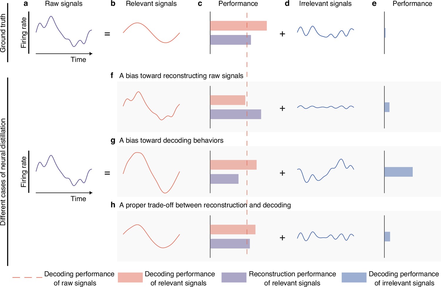
Semantic illustration of extracting and validating behaviorally relevant signals.
(a–e) The ideal decomposition of raw signals. (a) The temporal neuronal activity of raw signals, where x-axis denotes time, and y-axis represents firing rate. Raw signals are decomposed to relevant (b) and irrelevant (d) signals. The red dotted line indicates the decoding performance of raw signals. The red and blue bars represent the decoding performance of relevant and irrelevant signals. The purple bar represents the reconstruction performance of relevant signals, which measures the neural similarity between generated signals and raw signals. The longer the bar, the larger the performance. The ground truth of relevant signals decodes information perfectly (c, red bar) and is similar to raw signals to some extent (c, purple bar), and the ground truth of irrelevant signals contains little behavioral information (e, blue bar). (f–h) Three different cases of behaviorally relevant signals distillation. (f) When the model is biased toward generating relevant signals that are similar to raw signals, it will achieve high reconstruction performance, but the decoding performance will suffer due to the inclusion of too many irrelevant signals. As it is difficult for models to extract complete relevant signals, the residuals will also contain some behavioral information. (g) When the model is biased toward generating signals that prioritize decoding over similarity to raw signals, it will achieve high decoding performance, but the reconstruction performance will be low. Meanwhile, the residuals will contain a significant amount of behavioral information. (h) When the model balances the trade-off of decoding and reconstruction capabilities of relevant signals, both decoding and reconstruction performance will be good, and the residuals will only contain a little behavioral information.
Figure 1—figure supplement 1
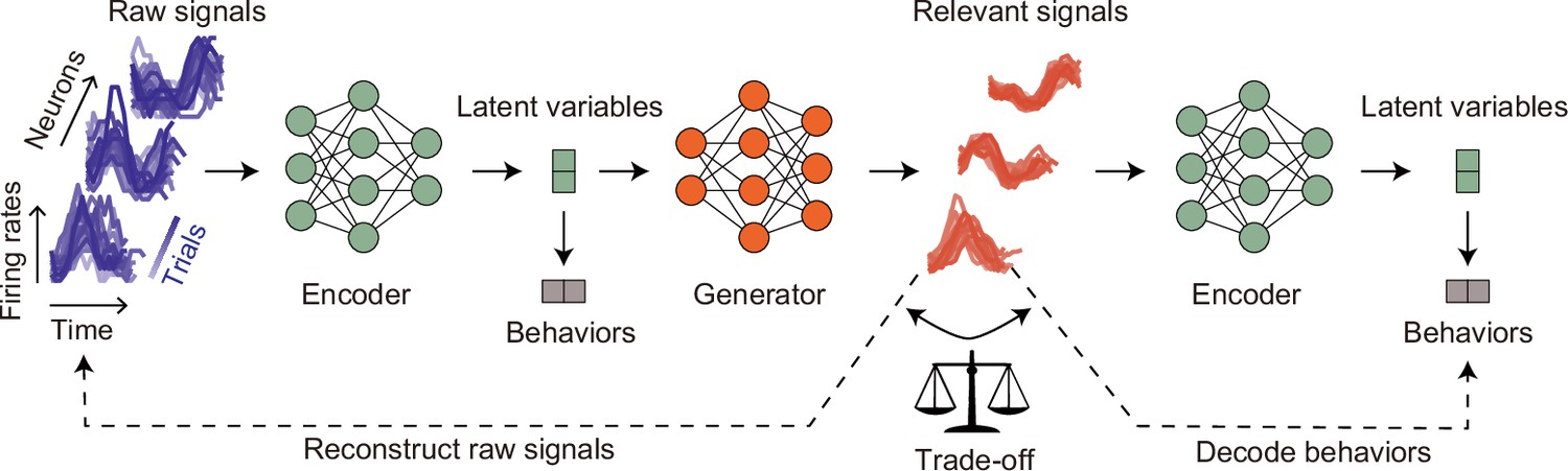
Semantic overview of distill-variational autoencoder (d-VAE).
On the left, we present a set of raw signal examples (depicted by purple lines). The input neural signals fed into the d-VAE consist of single time step samples. Initially, the encoder compresses these input signals into latent variables. We constrain latent variables to decode behaviors to preserve behavioral information. Subsequently, these latent variables are transmitted to the generator, which produces behaviorally relevant signals (depicted by red lines). To maintain the underlying neuronal properties, we constrain these generated signals to resemble the raw signals closely. At this juncture, relying solely on the constraint for signal resemblance to raw signals makes it challenging to determine the extent of irrelevant signals present within the generated relevant signals. To tackle this hurdle, we introduce the generated signals back into the encoder. We then impose constraints on the resultant latent variables to decode behaviors. This approach is rooted in the assumption that irrelevant signals function as noise relative to relevant signals. Consequently, an excessive presence of irrelevant signals within the generated signals would lead to a degradation in their decoding performance. In essence, there exists a trade-off relationship between the decoding performance and the reconstruction performance of the generated signals. By striking a balance between these two constraints, we can effectively extract behaviorally relevant signals.
Figure 1—figure supplement 2
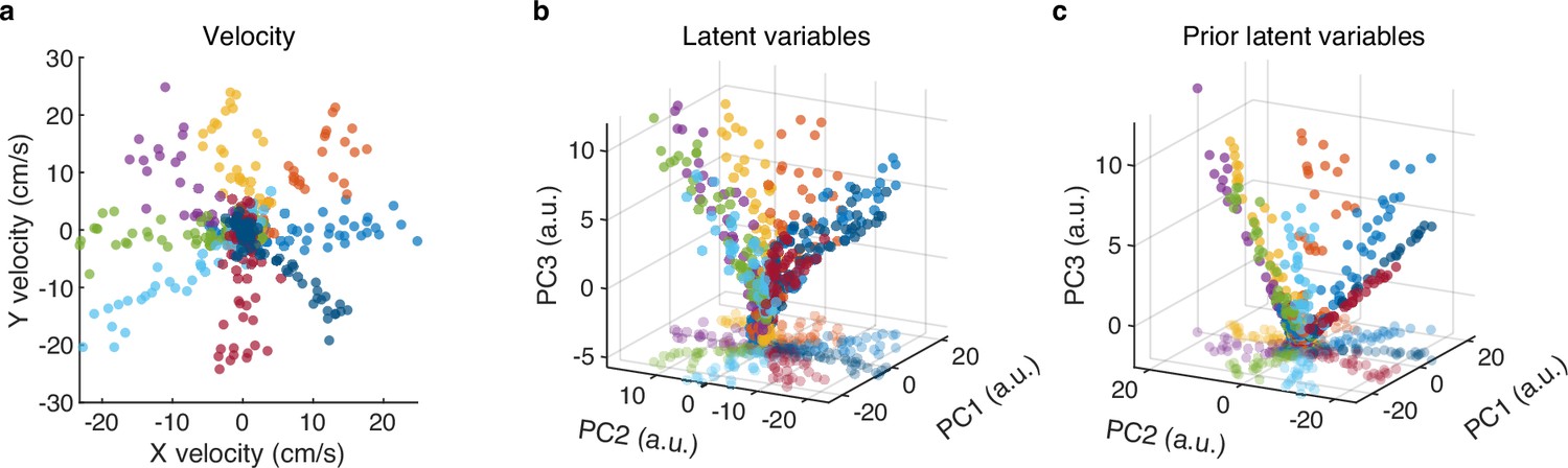
Visualization of latent variables.
(a) The velocity samples of onefold test data. Different colors denote different directions of the eight-direction center-out. (b) The distribution plot of the top three principal components (PCs) of latent variables. The points on the bottom plane represent the two-dimensional projections of the three-dimensional data. (c) The distribution plot of the top three PCs of learned prior latent variables. We can see that the distribution of prior latent variables closely resembles that of latent variables, thus illustrating the effectiveness of the Kullback-Leibler (KL) divergence.
Figure 2 with 1 supplement
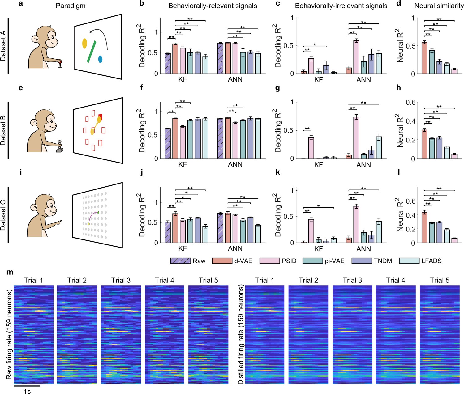
Evaluation of separated signals.
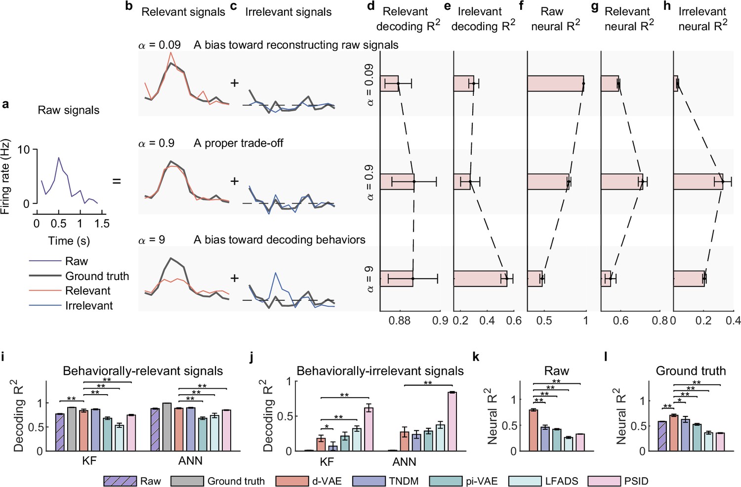
(a–d) Results for dataset A. (a) The obstacle avoidance paradigm. (b) The decoding between true velocity and predicted velocity of raw signals (purple bars with slash lines) and behaviorally relevant signals obtained by distill-variational autoencoder (d-VAE) (red), PSID (pink), pi-VAE (green), TNDM (blue), and LFADS (light green). Error bars denote mean ± standard deviation (s.d.) across five cross-validation folds. Asterisks represent significance of Wilcoxon rank-sum test with ∗p<0.05, ∗∗p<0.01. (c) Same as (b), but for behaviorally irrelevant signals obtained by five different methods. (d) The neural similarity () between raw signals and behaviorally relevant signals extracted by d-VAE, PSID, pi-VAE, TNDM, and LFADS. Error bars represent mean ± s.d. across five cross-validation folds. Asterisks indicate significance of Wilcoxon rank-sum test with ∗∗p<0.01. (e–h and i–l). Same as (a–d), but for dataset B with the center-out paradigm (e) and dataset C with the self-paced reaching paradigm (i). (m) The firing rates of raw signals and distilled signals obtained by d-VAE in five held-out trials under the same condition of dataset B.
Figure 2—figure supplement 1
Evaluation of separated signals on the synthetic dataset.
(a) The temporal neuronal activity of raw signals (the purple line) of an example test trial, which is decomposed into relevant (b) and irrelevant (c) signals. (b) Relevant signals (red lines) extracted by distill-variational autoencoder (d-VAE) under three distillation cases, where bold gray lines represent ground truth relevant signals. The hyperparameter is very important to extracting behaviorally relevant signals, which balances the trade-off between reconstruction loss and decoding loss. Results show that when , the relevant signals are too similar to raw signals but not similar to ground truth; when , the relevant signals are well similar to the ground truth; when , the relevant signals are not similar to the ground truth. (c) Same as (b), but for irrelevant signals (blue lines). Notably, when , some useful signals are left in irrelevant signals. (d) The decoding of distilled relevant signals of three cases. Error bars indicate mean ± standard deviation (s.d.) across five cross-validation folds. Results demonstrate that decoding increases as increases. (e) Same as (d), but for irrelevant signals. Notably, when , irrelevant signals will contain large behavioral information. (f) The neural similarity between relevant and raw signals. Results show that the neural decreases as increases. (g) The neural between relevant signals and the ground truth of relevant signals. Results show that d-VAE can utilize a proper trade-off to extract effective relevant signals that are similar to the ground truth. (h) The neural between irrelevant signals and the ground truth of irrelevant signals. Results show that d-VAE can utilize a proper trade-off to remove effective irrelevant signals that are similar to the ground truth. (i) The decoding between true velocity and predicted velocity of raw signals (purple bars with slash lines), the ground truth signals (gray) and behaviorally relevant signals obtained by d-VAE (red), PSID (pink), pi-VAE (green), TNDM (blue), and LFADS (light green). Error bars denote mean ± standard deviation (s.d.) across five cross-validation folds. Asterisks represent significance of Wilcoxon rank-sum test with ∗p<0.01, ∗∗p<0.01. (j) Same as (i), but for irrelevant signals. (k) The neural between generated relevant signals and raw signals. (l) Same as (k), but for the ground truth of relevant signals.
Figure 3 with 2 supplements
The effect of irrelevant signals on analyzing neural activity at the single-neuron level.
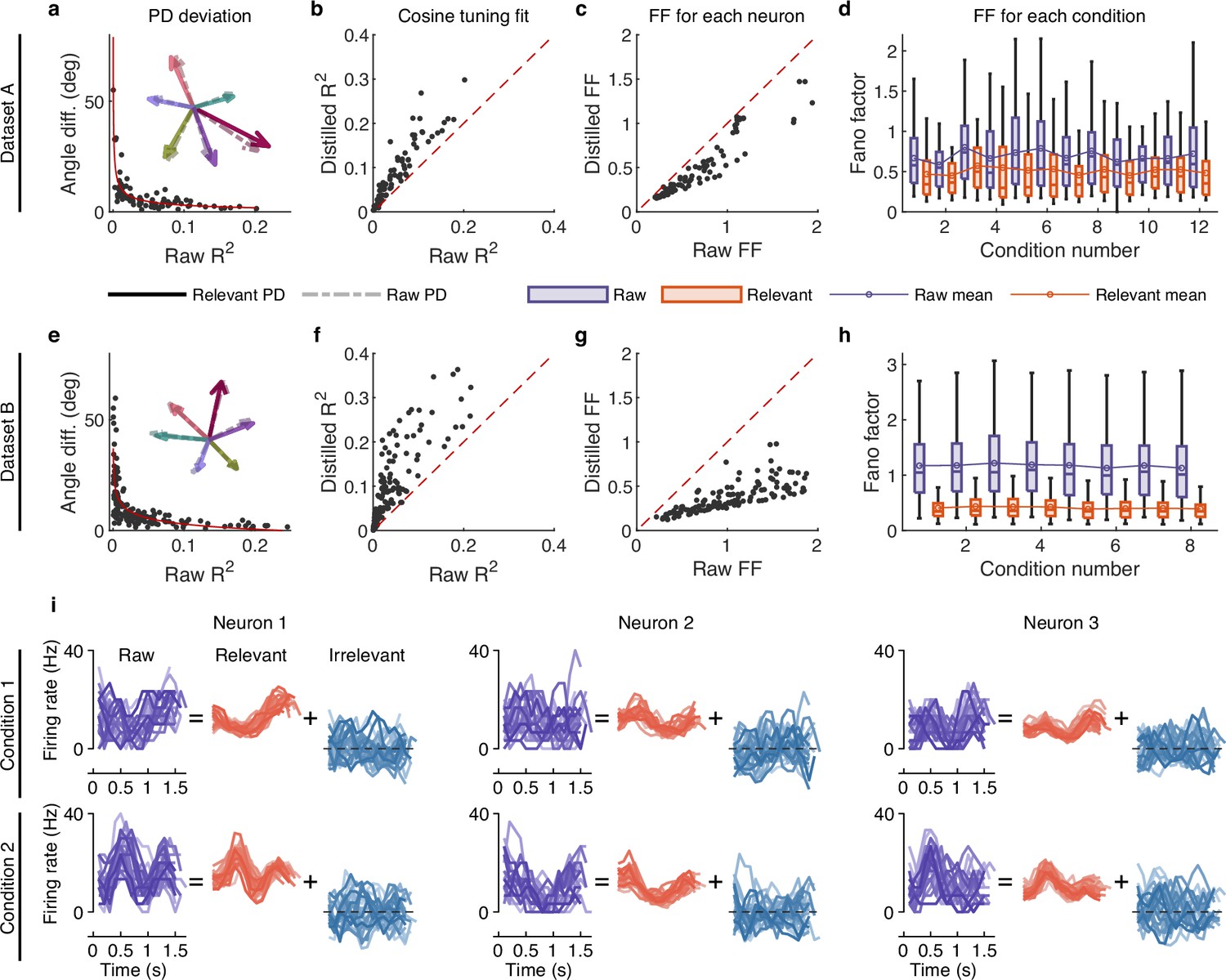
(a–d) Results for dataset A. (a) The angle difference (AD) of preferred direction (PD) between raw and distilled signals as a function of the of raw signals. When employing to characterize neurons, it indicates the extent to which neuronal activity is explained by the linear encoding model. Smaller neurons have a lower capacity for linearly tuning (encoding) behaviors, while larger neurons have a higher capacity for linearly tuning (encoding) behaviors. Each black point represents a neuron (n=90). The red curve is the fitting curve between and AD. Five example larger neurons’ PDs are shown in the inset plot, where the solid and dotted line arrows represent the PDs of relevant and raw signals, respectively. (b) Comparison of the cosine tuning fit () before and after distillation of single neurons (black points), where the x-axis and y-axis represent neurons’ of raw and distilled signals, respectively. (c) Comparison of neurons’ Fano factor (FF) averaged across conditions of raw (x-axis) and distilled (y-axis) signals, where FF is used to measure the neuronal variability of different trials in the same condition. (d) Boxplots of raw (purple) and distilled (red) signals under different conditions for all neurons (12 conditions). Boxplots represent medians (lines), quartiles (boxes), and whiskers extending to ±1.5 times the interquartile range. The broken lines represent the mean FF across all neurons. (e–h) Same as (a–d), but for dataset B (n=159, 8 conditions). (i) Example of three neurons’ raw firing activity decomposed into behaviorally relevant and irrelevant parts using all trials under two conditions (2 of 8 directions) in held-out test sets of dataset B.
Figure 3—figure supplement 1
The effect of irrelevant signals on relevant signals at the single-neuron level.
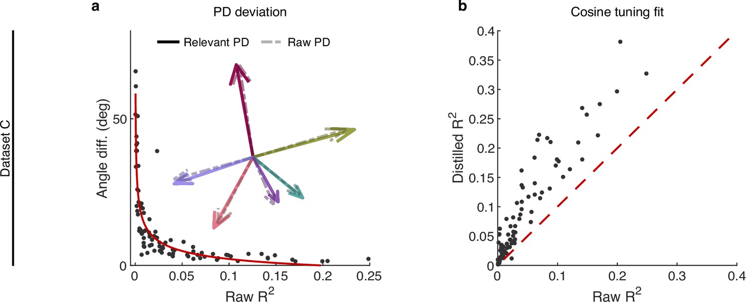
(a, b) Same as Figure 3, but for dataset C. (a) The angle difference (AD) of preferred direction (PD) between raw and distilled signals as a function of the of raw signals. Each black point represents a neuron (n=91). The red curve is the fitting curve between and AD. Five example larger neurons’ PDs are shown in the inset plot, where the solid line arrows represent the PD of relevant signals, and the dotted line arrows represent the PDs of raw signals. (b) Comparison of the cosine tuning fit () before and after distillation of single neurons (black points), where the x-axis and y-axis represent neurons’ of raw and distilled signals.
Figure 3—figure supplement 2
The firing activity of example neurons.
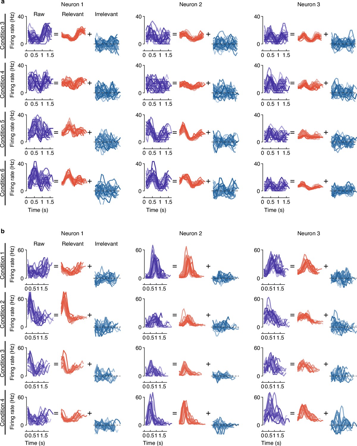
(a) Example of three neurons’ raw firing activity decomposed into behaviorally relevant and irrelevant parts using all trials in held-out test sets for four conditions (4 of 8 directions) of center-out reaching task. (b) Example of three neurons’ raw firing activity decomposed into behaviorally relevant and irrelevant parts using all trials in held-out test sets for four conditions (4 of 12 conditions) of obstacle avoidance task.
Figure 4 with 4 supplements
The effect of irrelevant signals on analyzing neural activity at the population level.
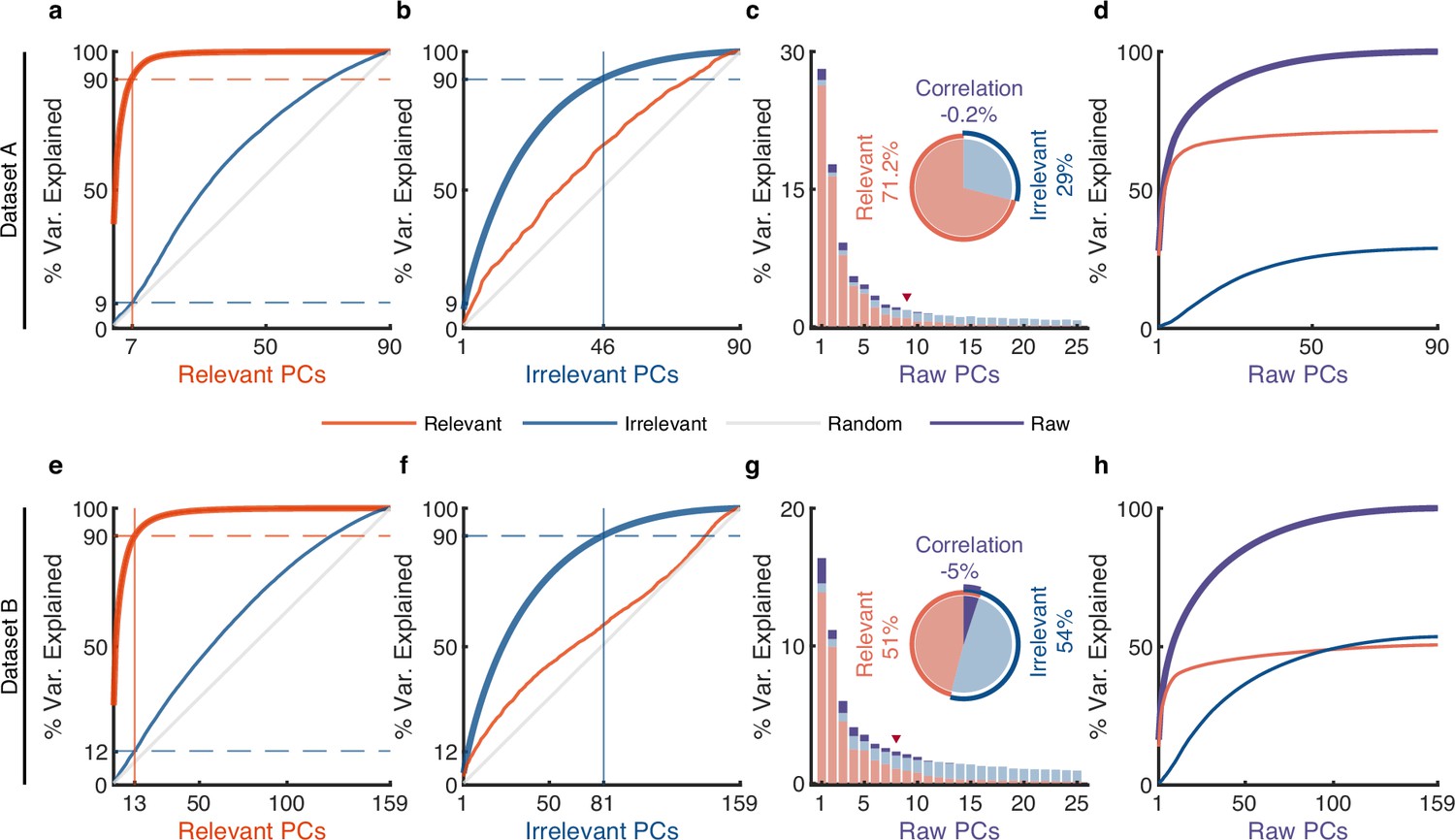
(a–d) Results for dataset A. (a) The cumulative variance curve for different signals, including relevant signals (red), irrelevant signals (blue), and random Gaussian noise (gray, representing the chance level), projected onto the principal components (PCs) of relevant signals. Specifically, principal component analysis (PCA) is applied to relevant signals to get relevant PCs. Subsequently, the three types of signals are projected onto these relevant PCs to obtain their respective cumulative variance curves. The thick lines represent the cumulative variance explained for the signals on which PCA has been performed, while the thin lines represent the variance explained by those PCs for other signals. The horizontal dotted lines represent the percentage of variance explained. The vertical lines indicate the number of dimensions that accounted for 90% of the variance in behaviorally relevant (left) and irrelevant (right) signals. For convenience, we defined the PC subspace describing the top 90% variance as the primary subspace and the subspace capturing the last 10% variance as the secondary subspace. (b) Same as (a), but for irrelevant PCs. (c) The composition of raw signals and each raw PC. Specifically, PCA is applied to the raw signals to obtain raw PCs. Then, the relevant and irrelevant signals are projected onto these raw PCs to determine the variance of the raw signals explained by each type of signal. The bar plot shows the composition of each raw PC. The inset pie plot shows the overall proportion of raw signals, where red, blue, and purple colors indicate relevant signals, irrelevant signals, and the correlation between relevant and relevant signals. The PC marked with a red triangle indicates the last PC where the variance of relevant signals is greater than or equal to that of irrelevant signals. (d) The cumulative variance explained by raw PCs for different signals, where the thick line represents the cumulative variance explained for raw signals (purple), while the thin line represents the variance explained for relevant (red) and irrelevant (blue) signals. (e–h) Same as (a–d), but for dataset B.
Figure 4—figure supplement 1
The effect of irrelevant signals on analyzing neural activity at the population level.
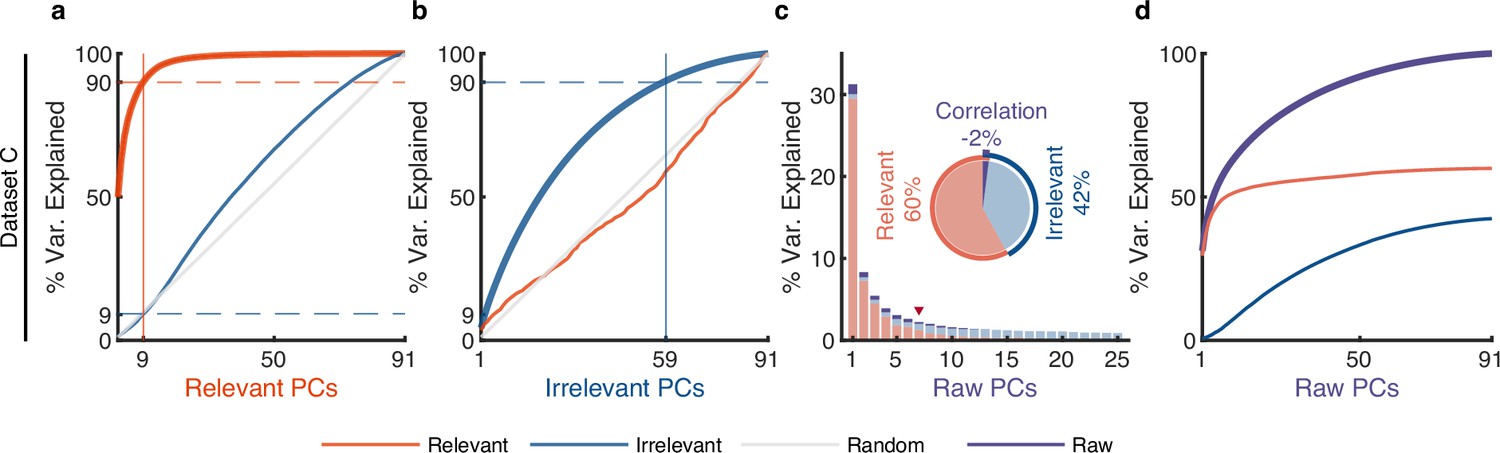
(a–d) Same as Figure 4, but for dataset C. (a) The cumulative variance curve for different signals, including relevant signals (red), irrelevant signals (blue), and random Gaussian noise (gray, representing the chance level), projected onto the principal components (PCs) of relevant signals. Specifically, principal component analysis (PCA) is applied to relevant signals to get relevant PCs. Subsequently, the three types of signals are projected onto these relevant PCs to obtain their respective cumulative variance curves. The thick lines represent the cumulative variance explained for the signals on which PCA has been performed, while the thin lines represent the variance explained by those PCs for other signals. The horizontal dotted lines represent the percentage of variance explained. The vertical lines indicate the number of dimensions that accounted for 90% of the variance in behaviorally relevant (left) and irrelevant (right) signals. For convenience, we defined the PC subspace describing the top 90% variance as the primary subspace and the subspace capturing the last 10% variance as the secondary subspace. (b) Same as (a), but for irrelevant PCs. (c) The composition of raw signals and each raw PC. Specifically, PCA is applied to the raw signals to obtain raw PCs. Then, the relevant and irrelevant signals are projected onto these raw PCs to determine the variance of the raw signals explained by each type of signal. The bar plot shows the composition of each raw PC. The inset pie plot shows the overall proportion of raw signals, where red, blue, and purple colors indicate relevant signals, irrelevant signals, and the correlation between relevant and relevant signals. The PC marked with a red triangle indicates the last PC where the variance of relevant signals is greater than or equal to that of irrelevant signals. (d) The cumulative variance explained by raw PCs for different signals, where the thick line represents the cumulative variance explained for raw signals (purple), while the thin line represents the variance explained for relevant (red) and irrelevant (blue) signals.
Figure 4—figure supplement 2
The effect of irrelevant signals obtained by pi-VAE on analyzing neural activity at the population level.
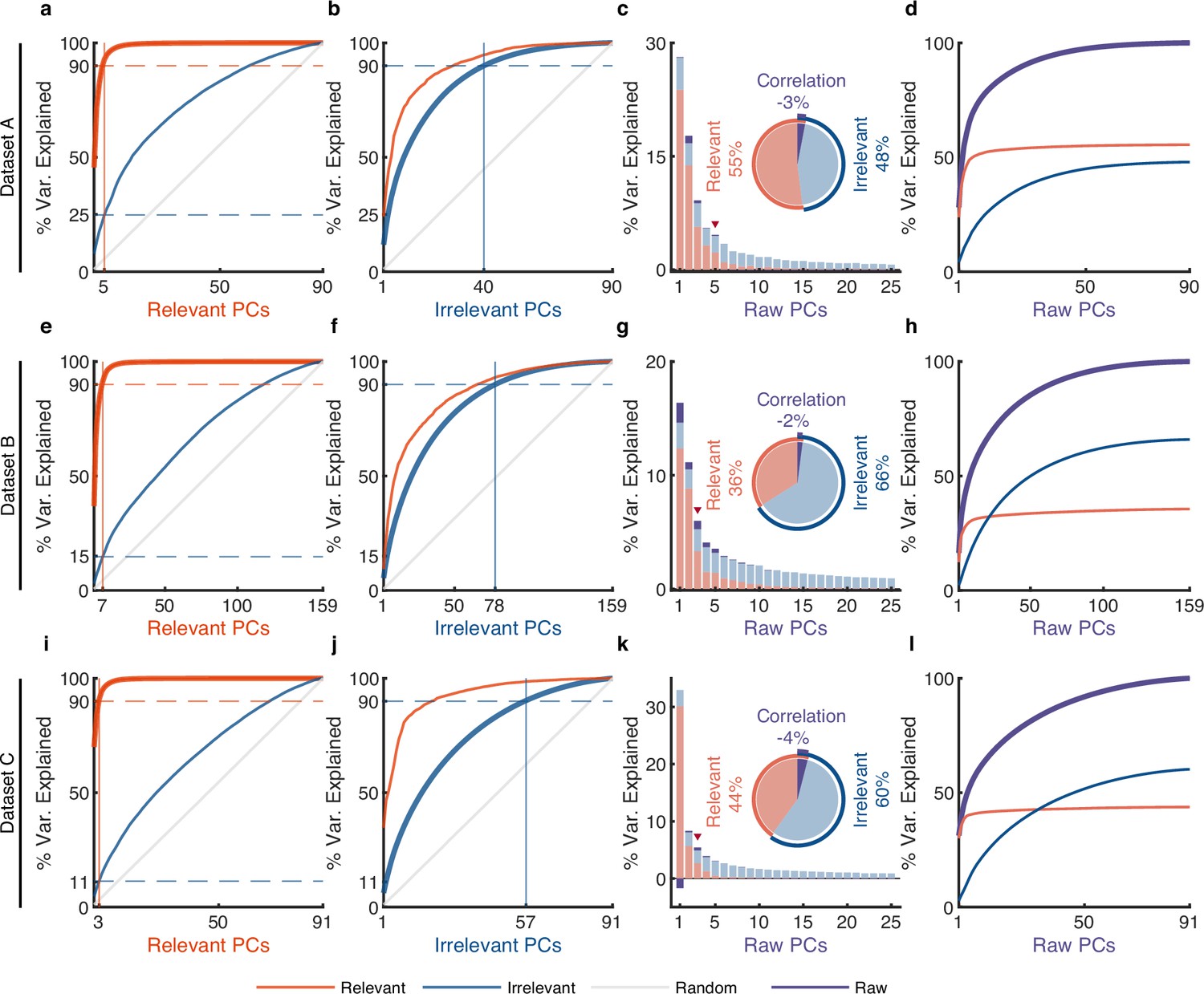
(a–l) Same as Figure 4 and Figure 4—figure supplement 1, but for pi-VAE. (a) The cumulative variance curve for different signals, including relevant signals (red), irrelevant signals (blue), and random Gaussian noise (gray, representing the chance level), projected onto the principal components (PCs) of relevant signals. Specifically, principal component analysis (PCA) is applied to relevant signals to get relevant PCs. Subsequently, the three types of signals are projected onto these relevant PCs to obtain their respective cumulative variance curves. The thick lines represent the cumulative variance explained for the signals on which PCA has been performed, while the thin lines represent the variance explained by those PCs for other signals. The horizontal dotted lines represent the percentage of variance explained. The vertical lines indicate the number of dimensions that accounted for 90% of the variance in behaviorally relevant (left) and irrelevant (right) signals. For convenience, we defined the PC subspace describing the top 90% variance as the primary subspace and the subspace capturing the last 10% variance as the secondary subspace. (b) Same as (a), but for irrelevant PCs. (c) The composition of raw signals and each raw PC. Specifically, PCA is applied to the raw signals to obtain raw PCs. Then, the relevant and irrelevant signals are projected onto these raw PCs to determine the variance of the raw signals explained by each type of signal. The bar plot shows the composition of each raw PC. The inset pie plot shows the overall proportion of raw signals, where red, blue, and purple colors indicate relevant signals, irrelevant signals, and the correlation between relevant and relevant signals. The PC marked with a red triangle indicates the last PC where the variance of relevant signals is greater than or equal to that of irrelevant signals. (d) The cumulative variance explained by raw PCs for different signals, where the thick line represents the cumulative variance explained for raw signals (purple), while the thin line represents the variance explained for relevant (red) and irrelevant (blue) signals. (e–h, i–l) Same as (a–d), but for datasets B and C.
Figure 4—figure supplement 3
The rotational dynamics of raw, relevant, and irrelevant signals.
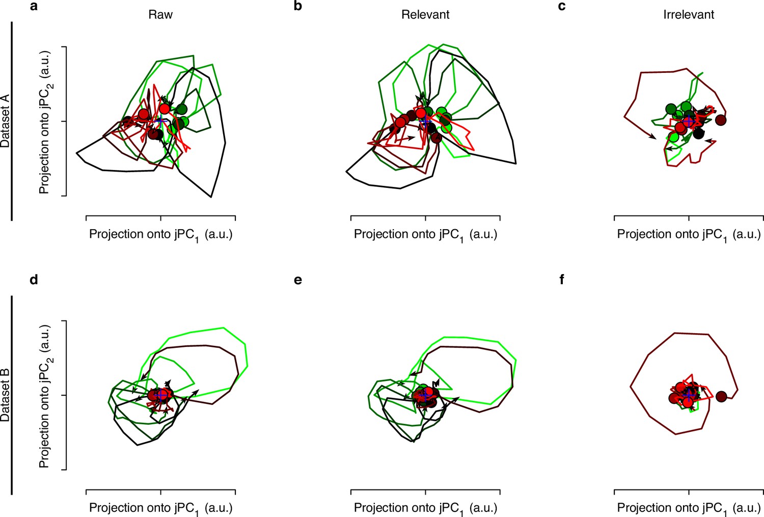
Datasets A and B have 12 and 8 conditions, respectively. We get the trial-averaged neural responses for each condition, then apply jPCA to raw, relevant, and irrelevant signals to get the top two jPC, respectively. (a) The rotational dynamics of raw neural signals. (b) The rotational dynamics of relevant signals obtained by distill-variational autoencoder (d-VAE). (c) The rotational dynamics of irrelevant signals obtained by d-VAE. We can see that the rotational dynamics of behaviorally relevant signals are similar to that of raw signals, but the rotational dynamics of behaviorally irrelevant signals are irregular. (d–f) Same as (a–c), but for dataset B.
Figure 4—figure supplement 4
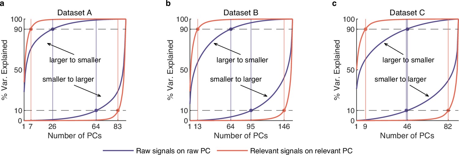
The cumulative variance curve for raw and behaviorally relevant signals.
(a) The cumulative variance curve for raw (purple) and behaviorally relevant (red) signals on their respective principal components (PCs) on dataset A (n=90). Two upper left corner curves denote the variance accumulation from larger to smaller variance PCs. Two lower right corner curves indicate accumulation from smaller to larger variance PCs. The horizontal lines represent the 10% and 90% variance explained. The vertical lines indicate the number of dimensions accounted for the last 10% and top 90% of the variance of behaviorally relevant (red) and raw (purple) signals. Here, we call the subspace composed of PCs capturing the top 90% variance the primary subspace, and the subspace composed of PCs capturing the last 10% variance the secondary subspace. We can see that the dimensionality of the primary subspace of raw signals is significantly higher than that of relevant signals, indicating that irrelevant signals make us overestimate the neural dimensionality. (b, c) Same as (a), but for datasets B (n=159) and C (n=91).
Figure 5 with 2 supplements
Smaller neurons encode rich behavioral information in complex nonlinear ways.
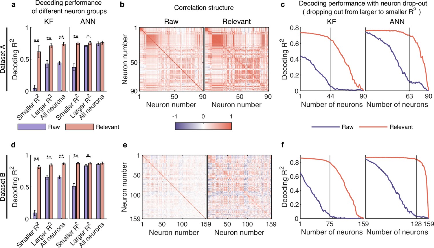
(a–c) Results for dataset A. (a) The comparison of decoding performance between raw (purple) and distilled signals (red) with different neuron groups, including smaller neuron (<=0.03), larger neuron (>0.03), and all neurons. Error bars indicate mean ± standard deviation (s.d.) across five cross-validation folds. Asterisks denote significance of Wilcoxon rank-sum test with ∗p<0.01, ∗∗p<0.01. (b) The correlation matrix of all neurons of raw (left) and behaviorally relevant (right) signals. Neurons are ordered to highlight correlation structure (details in Methods). (c) The decoding performance of Kalman filter (KF) (left) and artificial neural network (ANN) (right) with neurons dropped out from larger to smaller . The vertical gray line indicates the number of dropped neurons at which raw and behaviorally relevant signals have the greatest performance difference. (d–f) Same as (a–c), but for dataset B.
Figure 5—figure supplement 1
Neural responses usually considered to contain little information actually encode rich behavioral information in complex nonlinear ways.
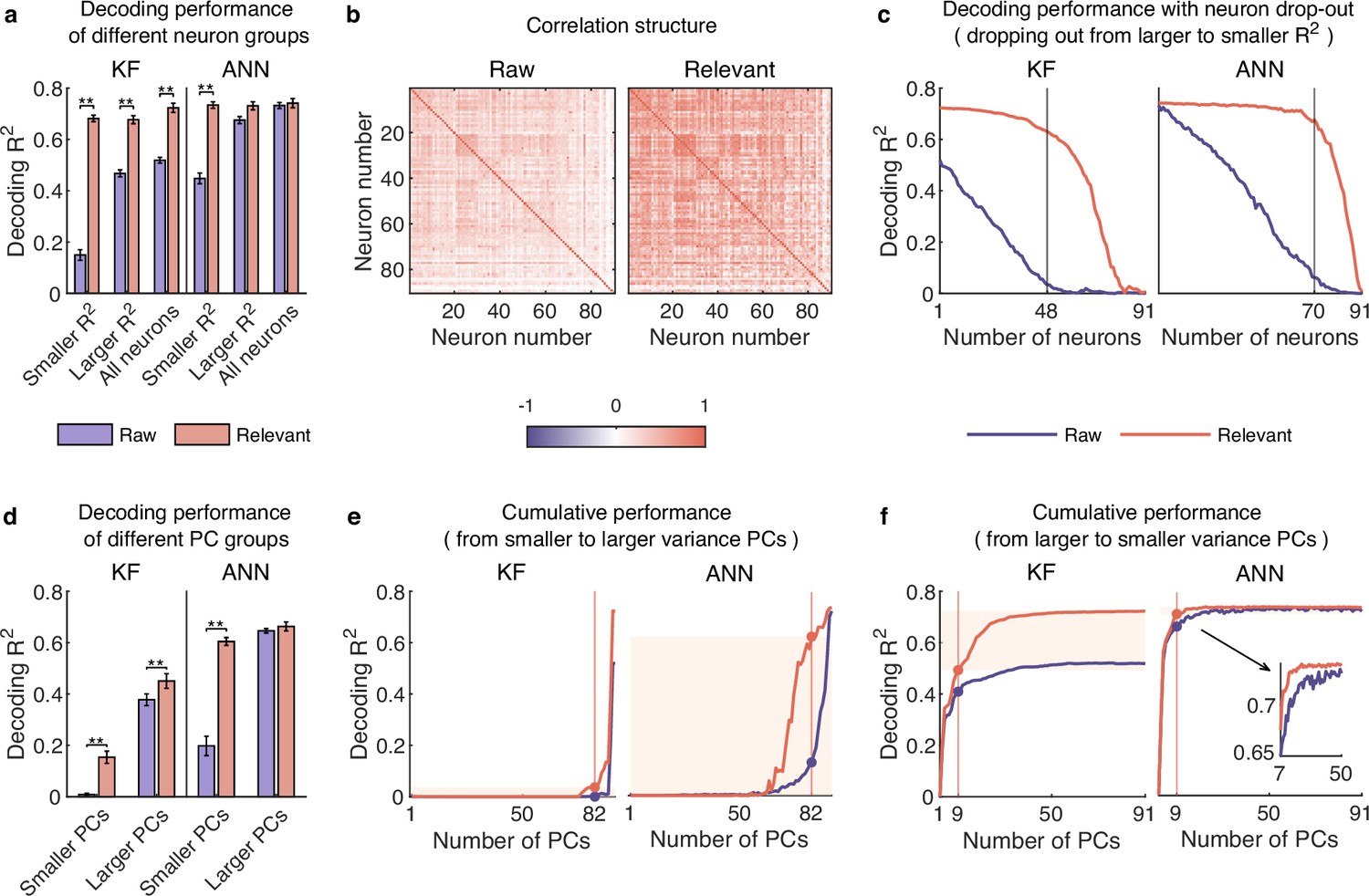
(a–c) Same as Figure 5, but for dataset C (n=91). (d–f) Same as Figure 6, but for dataset C. (a) The comparison of decoding performance between raw (purple) and distilled signals (red) with different neuron groups, including smaller neuron (<=0.03), larger neuron (>0.03), and all neurons. Error bars indicate mean ± standard deviation (s.d.) across cross-validation folds. Asterisks denote significance of Wilcoxon rank-sum test with ∗p<0.05, ∗∗p<0.01. (b) The correlation matrix of all neurons of raw and behaviorally relevant signals. (c) The decoding performance of Kalman filter (KF) (left) and artificial neural network (ANN) (right) with neurons dropped out from larger to smaller . The vertical gray lines indicate the number of dropped neurons at which raw and behaviorally relevant signals have the greatest performance difference. (d) The comparison of decoding performance between raw (purple) and distilled signals (red) composed of different raw-principal component (PC) groups, including smaller variance PCs (the proportion of irrelevant signals that make up raw PCs is higher than that of relevant signals), larger variance PCs (the proportion of irrelevant signals is lower than that of relevant ones). Error bars indicate mean ± s.d. across five cross-validation folds. Asterisks denote significance of Wilcoxon rank-sum test with ∗p<0.05, ∗∗p<0.01. (e) The cumulative decoding performance of signals composed of cumulative PCs that are ordered from smaller to larger variance using KF (left) and ANN (right). The red patches indicate the decoding ability of the last 10% variance of relevant signals. (f) Same as (e), but PCs are ordered from larger to smaller variance. The red patches indicate the decoding gain of the last 10% variance signals of relevant signals superimposing on their top 90% variance signals.
Figure 5—figure supplement 2
Using synthetic data to demonstrate that conclusions are not a by-product of distill-variational autoencoder (d-VAE).
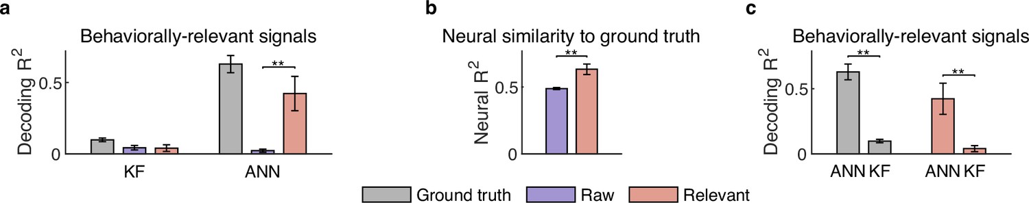
(a, b) These results are used to demonstrate that d-VAE can utilize the larger neurons to help the smaller neurons restore their original face. (a) The decoding of the ground truth (gray), raw signals (purple), and distilled relevant signals (red) of smaller neurons of synthetic data. Error bars indicate mean ± standard deviation (s.d.) (n=5 folds). Asterisks denote the significance of Wilcoxon rank-sum test with ∗∗p<0.01. We can see that the ground truth of smaller neurons contain a certain amount of behavioral information, but the behavioral information cannot be decoded from raw signals due to being covered by noise; d-VAE can indeed utilize the larger neurons to help the smaller neurons restore their damaged information. (b) The neural similarity of raw signals and relevant signals to ground truth of smaller neurons. We can see that d-VAE can obtain effective relevant signals that are more similar to the ground truth compared to raw signals. (c) The decoding of the ground truth (gray) and distilled relevant signals (red) of smaller neurons of synthetic data. These results are used to demonstrate that d-VAE cannot make the linear decoder achieve similar performance as the nonlinear decoder. We can see that Kalman filter (KF) is significantly inferior to artificial neural network (ANN) on ground truth signals. The KF decoding performance of the ground truth signals is notably low, leaving significant room for compensation by d-VAE. However, after processing with d-VAE, the KF decoding performance of distilled signals does not surpass its ground truth performance. The disparity between KF and ANN remains substantial. These results demonstrate that d-VAE cannot make signals that originally require nonlinear decoding linearly decodable.
Figure 6 with 1 supplement
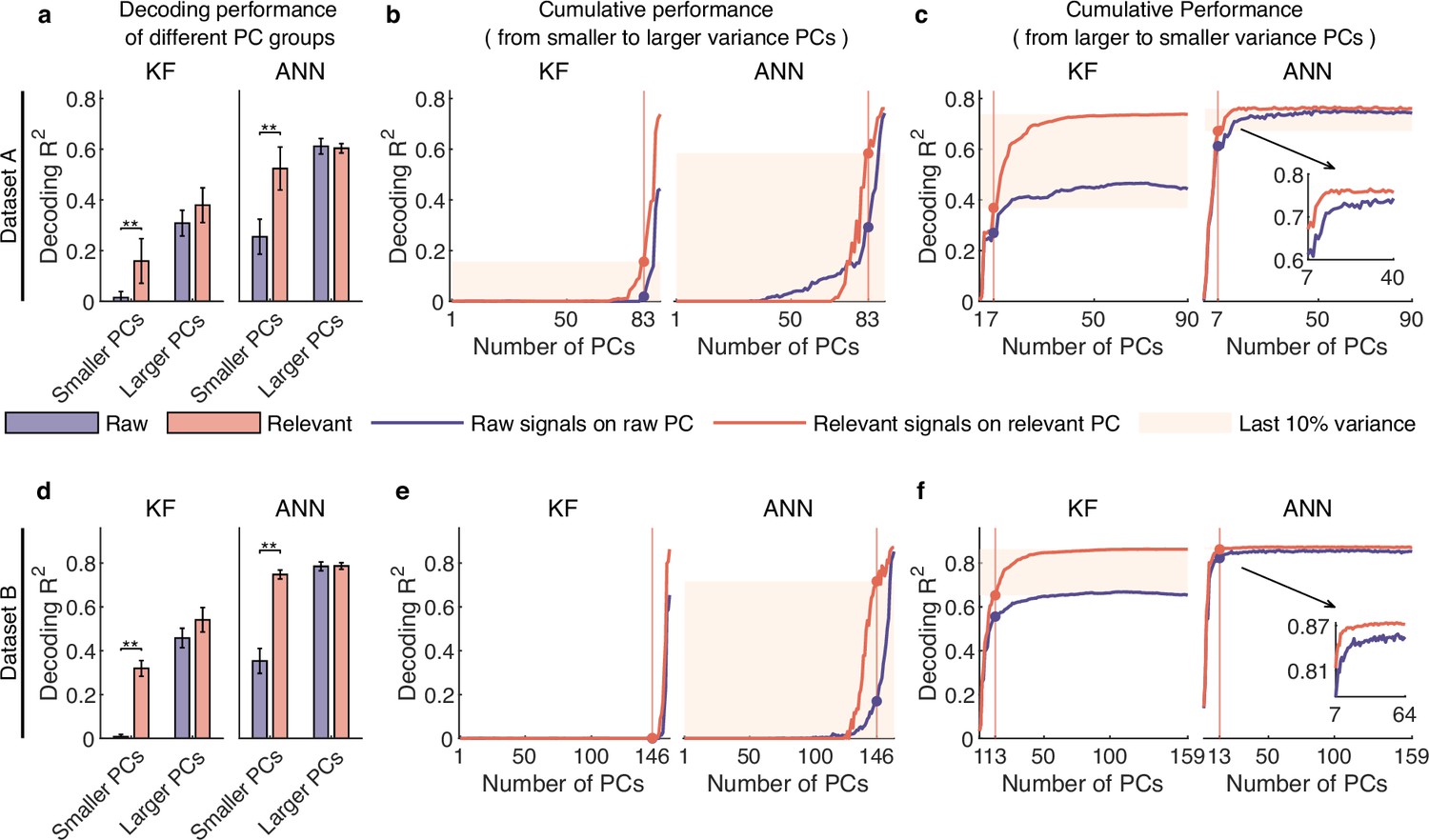
Signals composed of smaller variance principal components (PCs) encode rich behavioral information in complex nonlinear ways.
(a–c) Results for dataset A. (a) The comparison of decoding performance between raw (purple) and distilled signals (red) composed of different raw PC groups, including smaller variance PCs (the proportion of irrelevant signals that make up raw PCs is higher than that of relevant signals), larger variance PCs (the proportion of irrelevant signals is lower than that of relevant ones). Error bars indicate mean ± standard deviation (s.d.) across five cross-validation folds. Asterisks denote significance of Wilcoxon rank-sum test with ∗p<0.01, ∗∗p<0.01. (b) The cumulative decoding performance of signals composed of cumulative PCs that are ordered from smaller to larger variance using Kalman filter (KF) (left) and artificial neural network (ANN) (right). The red patches indicate the decoding ability of the last 10% variance of relevant signals. (c) The cumulative decoding performance of signals composed of cumulative PCs that are ordered from larger to smaller variance using KF (left) and ANN (right). The red patches indicate the decoding gain of the last 10% variance signals of relevant signals superimposing on their top 90% variance signals. The inset shows the partially enlarged plot for view clearly. (d–f) Same as (a–c), but for dataset B.
Figure 6—figure supplement 1
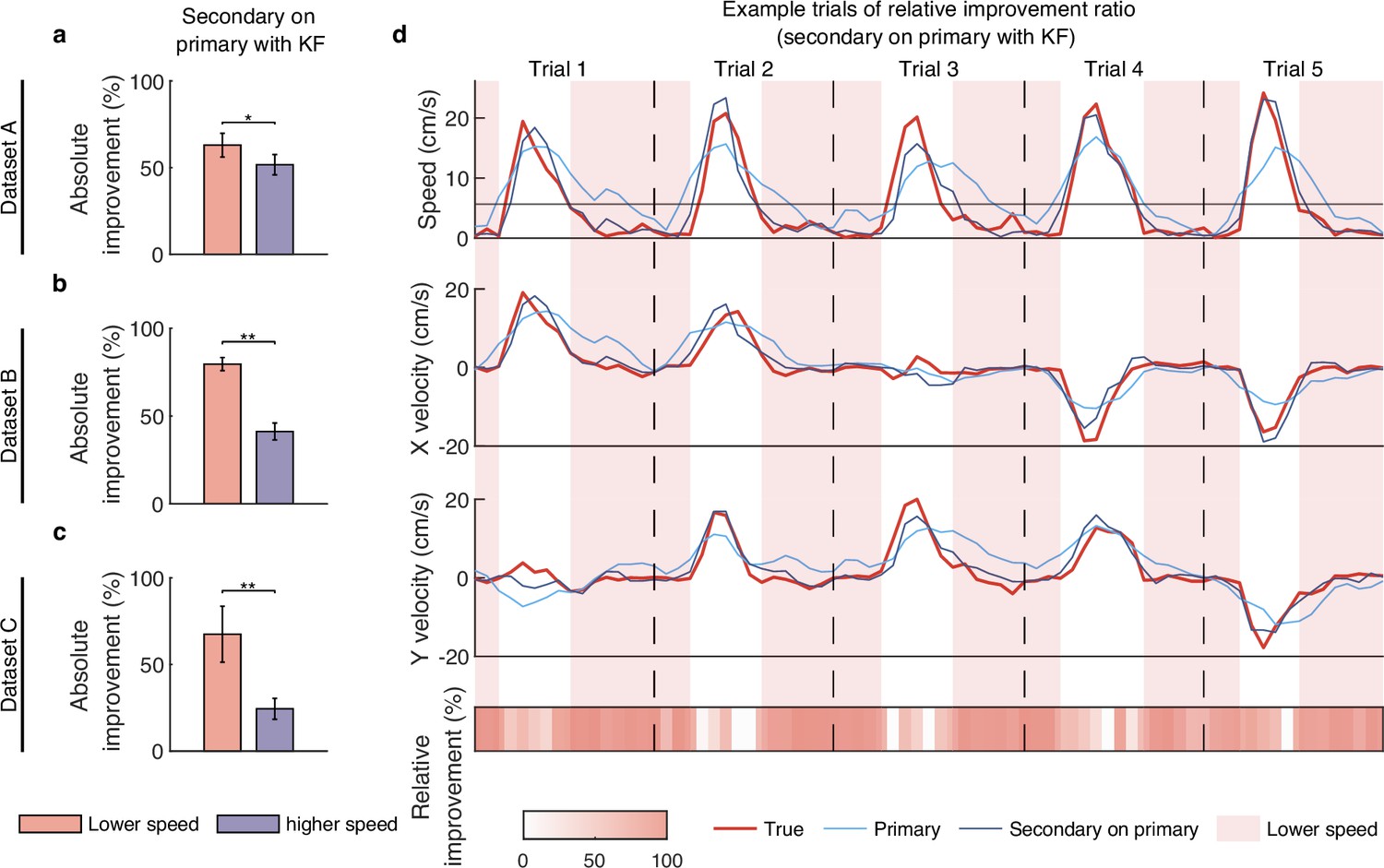
Smaller variance principal component (PC) signals preferentially improve lower-speed velocity.
(a) The comparison of absolute improvement ratio between lower-speed (red) and higher-speed (purple) velocity when superimposing secondary signals on primary signals with Kalman filter (KF) on dataset A. Error bars indicate mean ± standard deviation (s.d.) across five cross-validation folds. Asterisks denote significance of Wilcoxon rank-sum test with ∗p<0.05, ∗∗p<0.01. (b, c) Same as (a), but for datasets B and C. (d) The comparison of relative improvement ratio between lower-speed (red patch) and higher-speed (no patch) velocity when superimposing secondary signals on primary signals with KF on dataset B. The first-row plot shows five example trials’ speed profile of the decoded velocity using primary signals (light blue line) and full signals (dark blue line; superimposing secondary signals on primary signals) and the true velocity (red line). The black horizontal line denotes the speed threshold. The second and third-row plots are the same as the first-row plot, but for X and Y velocity. The fourth-row plot shows the relative improvement ratio for each point in trials.
Tables
Author response table 1
Decoding R2 of irrelevant signals.
| Dataset A | Dataset B | Dataset C | |
|---|---|---|---|
| Alpha = 0 | 0.065+-0.027 | 0.098+-0.037 | 0.071+-0.034 |
| Selected alpha | 0.105+-0.032 | 0.067+-0.031 | 0.095+-0.037 |
| Alpha = 0.9 | 0.220+-0.045 | 0.106+-0.044 | 0.182+-0.056 |
Author response table 2
Decoding R2 of behaviorally relevant signals obtained by d-VAE2.
| Dataset A | Dataset B | Dataset C | |
|---|---|---|---|
| KF | 0.706+-0.016 | 0.704+-0.039 | 0.860+-0.012 |
| ANN | 0.752+-0.010 | 0.738+-0.033 | 0.870+-0.009 |
Author response table 3
Neural R2 between generated signals and real behaviorally relevant signals.
| Alpha | 0.7 | 0.8 | 0.9 | 1 | 2 | 3 |
|---|---|---|---|---|---|---|
| d- | 0.720+- | 0.716+- | 0.712+- | 0.730+- | 0.736+- | 0.713+- |
| VAE | 0.014 | 0.028 | 0.023 | 0.021 | 0.009 | 0.013 |
| d- | 0.689+- | 0.693+- | 0.703+- | 0.720+- | 0.727+- | 0.679+- |
| VAE2 | 0.033 | 0.051 | 0.006 | 0.019 | 0.015 | 0.027 |
Additional files
Download links
A two-part list of links to download the article, or parts of the article, in various formats.
Downloads (link to download the article as PDF)
Open citations (links to open the citations from this article in various online reference manager services)
Cite this article (links to download the citations from this article in formats compatible with various reference manager tools)
Revealing unexpected complex encoding but simple decoding mechanisms in motor cortex via separating behaviorally relevant neural signals
eLife 12:RP87881.
https://doi.org/10.7554/eLife.87881.4


