Figures and data in Free volume theory explains the unusual behavior of viscosity in a non-confluent tissue during morphogenesis | eLife

Figures
Videos
Tables
Additional files

18 figures, 3 videos, 1 table and 1 additional file

Figures

Figure 1

Download asset Open asset

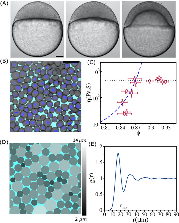
Structure and viscosity of non-confluent tissues.

(A) Bright-field single-plane images of an exemplary embryo of zebrafish before ( $t = - 60$ min), at the onset ( $t = 0$ min), and after blastoderm spreading ( $t = 60$ min). (B) Snapshot of 2D confocal sections at the 1st–2nd deep-cell layer of the blastoderm at $t = 60$ min. (A) and (B) are taken from Petridou et al., 2021. (C) Viscosity $η$ of zebrafish blastoderm as a function of $ϕ$ in a log-linear scale using the data from Petridou et al., 2021. The dashed line is the fit to Vogel–Fulcher–Tammann (VFT) equation. Note that $η$ does not change significantly beyond $ϕ \geq 0.87$ . (D) A typical snapshot taken from cell-based simulations for $ϕ = 0.93$ . Cells are colored according to their radii (in µm) (color bar shown on the right). (E) The pair correlation function, $g (r)$ , as a function of $r$ for $ϕ = 0.93$ . The vertical dashed line is the position of the first peak ( $r_{max} = 17.0 μ m$ ). The pair correlation function does not exhibit signs of long-range order. Scale bars in (A) is 100 µm and (B) is 50 µm.

Figure 2

Download asset Open asset

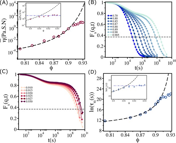
Saturation in viscosity and relaxation time.

(A) Effective viscosity $\bar{η}$ as a function of $ϕ$ , with the solid line being the fit to Vogel–Fulcher–Tammann (VFT) equation. The inset shows $\bar{η}$ at high $ϕ$ . The dashed line in the inset is the expected behavior assuming that the VFT relation holds at all $ϕ$ . (B) The self-intermediate scattering function $F_{s} (q, t)$ as a function of $t$ for $0.70 \leq ϕ \leq 0.905$ . The dashed line corresponds to $F_{s} (q, t) = \frac{1}{e}$ . (C) A similar plot for $ϕ > 0.905$ . (D) The logarithm of the relaxation time $τ_{α} (s)$ as a function of $ϕ$ . The VFT fit is given by the dashed line. The inset shows a zoomed-in view for $ϕ \geq ϕ_{S}$ . The error bars in (D) are calculated using the standard deviation of $τ_{α}$ for 24 independent simulations.

Figure 3

Download asset Open asset

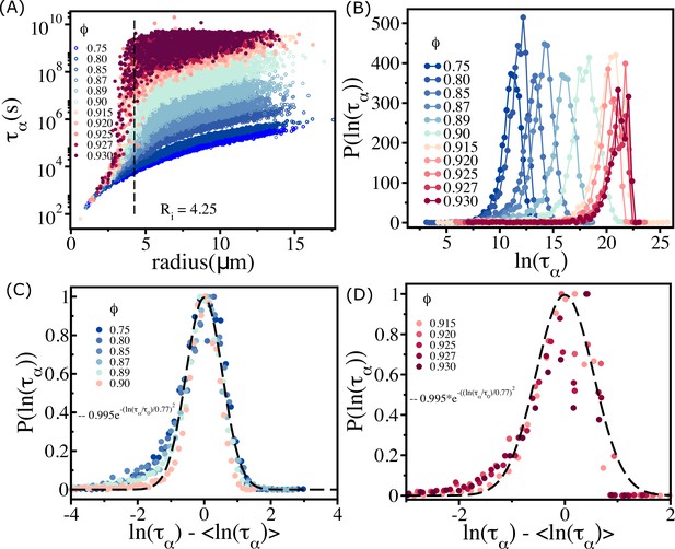
Spectrum of relaxation times.

(A) Scatter plot of relaxation times $τ_{α} (s)$ as a function of cell radius. From top to bottom, the plot corresponds to decreasing $ϕ$ . The vertical dashed line is for $R_{i} = 4.25 μ m$ , beyond which the $τ_{α}$ changes sharply at high packing fractions. (B) Histogram $P (\ln (τ_{α}))$ as a function of $\ln (τ_{α})$ . Beyond $ϕ = 0.90$ ( $ϕ_{S}$ ), the histogram peaks do not shift substantially towards a high $τ_{α}$ values. (C) For $ϕ \leq ϕ_{S} P (\ln (τ_{α}))$ (scaled by $P^{max} (\ln (τ_{α}))$ ) falls on a master curve, as described in the main text. (D) Same as (C) except the results are for $ϕ > 0.90$ . The data deviates from the Gaussian fit, shown by the dashed line.

Figure 4

Download asset Open asset

Density-dependent cell–cell overlap.

(A) Probability of overlap ( $h_{i j}$ ) between two cells, $P (h_{i j})$ , for various $ϕ$ values.The peak in the distribution function shifts to higher values as $ϕ$ increases. (B) Mean $⟨ h_{i j} ⟩ = \int d h_{i j} P (h_{i j})$ as a function of $ϕ$ . Inset shows a pictorial illustration of $h_{12}$ between two cells with radii $R_{1}$ and $R_{2}$ at a distance $r_{12}$ .

Figure 5

Download asset Open asset

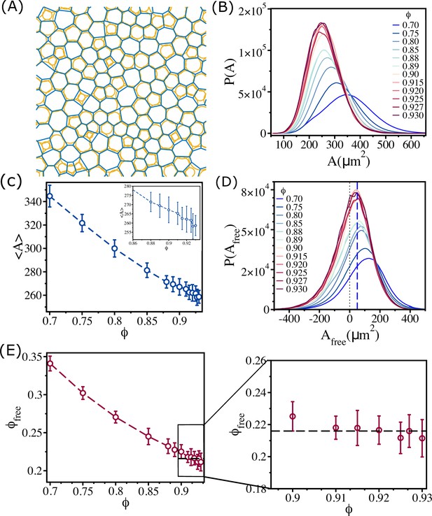
Changes in free area fraction with $ϕ$ .

(A) Voronoi tessellation of cells for $ϕ = 0.93$ for a single realization. The orange circles represent actual cell sizes. The blue polygons show the Voronoi cell size. (B) Distribution of Voronoi cell size $A$ as a function of $ϕ$ . (C) Mean Voronoi cell size $⟨ A ⟩$ as a function of $ϕ$ . A zoomed-in view for $ϕ > 0.860$ is shown in the inset. (D) Distribution of free area $P (A_{free})$ for all $ϕ$ . The vertical blue dashed line shows that the maximum in the distribution is at $A_{free} \sim 50 μ m^{2}$ . (E) Free area fraction $ϕ_{free}$ as a function of $ϕ$ . Note that $ϕ_{free}$ saturates beyond $ϕ = 0.90$ . An expanded view of the saturated region is shown in the right panel of (E). The error bars in (C) and (D) are the standard deviation in $⟨ A ⟩$ and $ϕ_{f r e e}$ , respectively, for 24 independent simulations.

Figure 6

Download asset Open asset

Relaxation in the polydisperse cell system is independent of the waiting time.

(A) $F_{s} (q, t)$ for $ϕ = 0.92$ at different waiting times ( $τ_{ω} = 10^{6} (s))$ . Regardless of the value of $τ_{ω}$ , all the $F_{s} (q, t)$ curves collapse onto a master curve. (B) Relaxation time, $\ln (τ_{α})$ , as a function of $τ_{ω}$ . Over a three orders of magnitude change in $t_{ω}$ , the variation in relaxation times is less than the sample-to-sample fluctuations, as shown by the error bar. The error bars in (B) are the standard deviation in $τ_{α}$ for 24 independent simulations.

Figure 7

Download asset Open asset

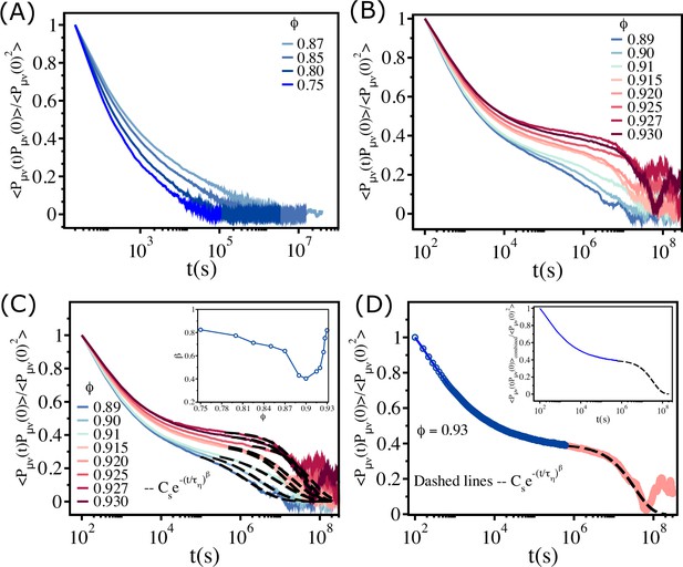
Fit of the stress–stress correlation functions to stretched exponential functions.

(A) The stress–stress correlation function $⟨ P_{μ ν} (t) P_{μ ν} (0) ⟩$ divided by the value at $t = 0 ⟨ P_{μ ν} (0)^{2} ⟩$ as a function of $t$ for $ϕ \in (0.75 - 0.87)$ . (B) Similar plot for $ϕ \in (0.89 - 0.93)$ . (C) The long time decay of $⟨ P_{μ ν} (t) P_{μ ν} (0) ⟩$ is fit to $C_{s} \exp [- (\frac{t}{τ_{η}})^{β}]$ , as shown by the dashed lines. The inset shows the dependence of $β$ on $ϕ$ . (D) The data that is fit using the stretched exponential function (black dashed line) is combined with the short time data (blue solid line), which is fit using the cubic spline function. The resulting fits produces a smooth curve ${⟨ P_{μ ν} (t) P_{μ ν} (0) ⟩}_{combined}$ , as shown in the inset.

Appendix 1—figure 1

Download asset Open asset

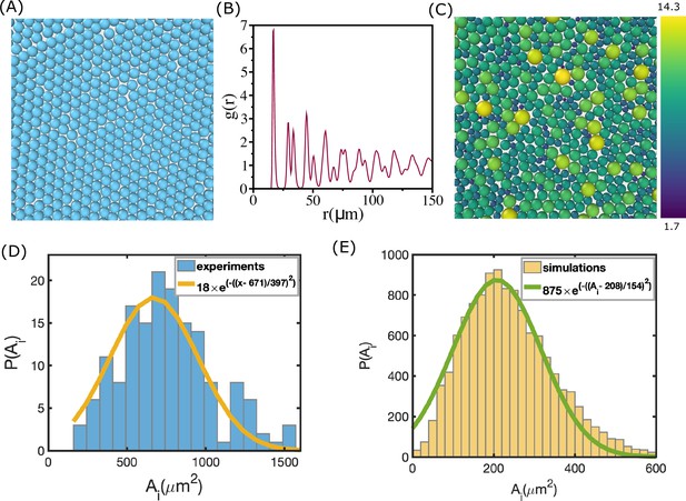
Area distribution of the cells.

(A) Simulation snapshot for monodisperse cell system. The number of cells in the two-dimensional periodic box is $N = 500$ . (B) Pair correlation function, $g (r)$ , as a function of $r$ . There is clear evidence of order, as reflected in the sharp peaks at regular intervals, which reflects the packing in (A). (C) A schematic picture of polydisperse cell system from the simulations. Color bar on the right shows the scale of radii in µm. There is no discernible order. (D) Distribution of cell area extracted from experiment during morphogenesis of zebrafish blastoderm (extracted from Fig. S2(A)) (Petridou et al., 2021). (E) Same as (D) except, $P (A_{i})$ , used in a typical simulation. Cell radii vary from 2 µm to 15 µm.

Appendix 2—figure 1

Download asset Open asset

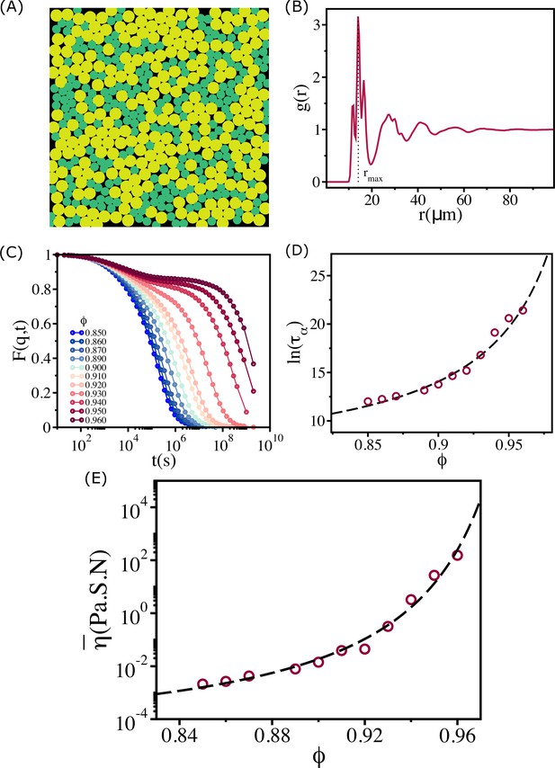
Structure and relaxation behavior for a binary mixture of cells.

(A) A typical simulation snapshot for binary mixture of cells at $ϕ = 0.93$ . (B) The corresponding pair correlation function, $g (r)$ , between all the cells. The vertical dashed line is at the first peak position ( $r_{m a x}$ ). (C) $F_{s} (q, t)$ , with $q = \frac{2 π}{r_{m a x}}$ , where $r_{m a x}$ is the location of the first peak in the $g (r)$ , as a function of time at various $ϕ$ values. (D) The logarithm of the relaxation time, $τ_{α}$ , as a function of $ϕ$ . Over the entire range of $ϕ$ , the increase in $τ_{α}$ is well fit by the Vogel–Fulcher–Tammann (VFT) (VFT) relation. Most importantly, the relaxation time does not saturate, which means the evolving tissue cannot be modeled using a 50:50 binary mixture. (E) Effective shear viscosity $\bar{η}$ as a function of $ϕ$ reflects the behavior of $τ$ as a function of $ϕ$ in (D).

Appendix 3—figure 1

Download asset Open asset

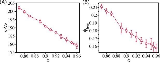
Free area decreases monotonically for the binary mixture of cells.

(A) Mean Voronoi cell size, $⟨ A ⟩$ , as a function of $ϕ$ for the 50:50 binary system. (B) The free area fraction, $ϕ_{f r e e}$ , as a function of $ϕ$ shows that $ϕ_{f r e e}$ decreases monotonically as $ϕ$ increases. The error bars in (B) are the standard deviation in $\phi_{free}$ for 24 independent simulations.

Appendix 4—figure 1

Download asset Open asset

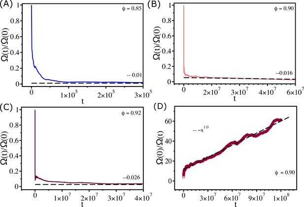
Measure of ergodicity.

(A) Ergodic measure $Ω (t)$ scaled by the value at $t = 0$ ( $Ω (0)$ ) as a function of $t$ for $ϕ = 0.85$ . (B, C) Similar plots for $ϕ = 0.90$ and $ϕ = 0.92$ , respectively. At long time, $Ω (t) / Ω (0)$ reach $0.01$ , $0.016$ , and $0.026$ for $ϕ = 0.85$ , $ϕ = 0.90$ , and $ϕ = 0.92$ , respectively. (D) $Ω (0) / Ω (t)$ as a function of $t$ for $ϕ = 0.90$ . The dashed line shows a linear fit. The time t is in second.

Appendix 5—figure 1

Download asset Open asset

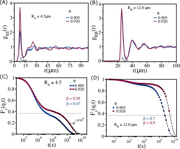
Cell size-dependent structures and dynamics.

(A) Radial distribution function $g_{S S} (r)$ between small-sized cells ( $R_{S} \leq 4.5 μ m$ ) at $ϕ = 0.905$ (blue) and $0.92$ (red). These values are greater than $ϕ_{s} \approx 0.90$ . (B) Same as (A) except the results are for $g_{B B} (r)$ between large cells ( $R_{B} \geq 12.0 μ m$ ). (C) $F_{s} (q, t)$ for cells with $R_{S} \leq 4.5 μ m$ at $ϕ = 0.905$ and $ϕ = 0.92$ . Note that even at these dense packings, the mobility of the smaller-sized cells is substantial, which is reflected in the time dependence of $F_{s} (q, t)$ . (D) $F_{s} (q, t)$ for cells with $R_{B} \geq 12.0 μ m$ at $ϕ = 0.905$ and $ϕ = 0.92$ . The black dashed lines are fits to stretched exponential functions, $F_{s} (q, t) \sim \exp (- (\frac{t}{τ_{α}})^{β})$ , where $τ_{α}$ is the relaxation time and $β$ is the stretching exponent. The dotted lines correspond to the value $F_{s} (q, t) = \frac{1}{e}$ .

Appendix 5—figure 2

Download asset Open asset

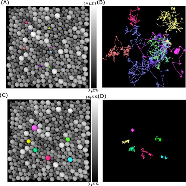
Simulation snapshot and trajectories for a few smaller- and bigger-sized cells.

(A) Cells ( $ϕ = 0.91$ ) are colored according to their sizes (gray colors). A few small-sized cells are shown in different colors (pink, blue, orange, purple, cyan, light purple, and yellow). (B) The corresponding trajectories are shown over the entire simulation time. (C) Similar plot as (A) but for a few bigger-sized cells shown in purple, yellow, light green, red, cyan, and green colors. (D) Same as (B) except the trajectories of the large-sized cells are highlighted. Clearly, the large cells are jammed.

Appendix 6—figure 1

Download asset Open asset

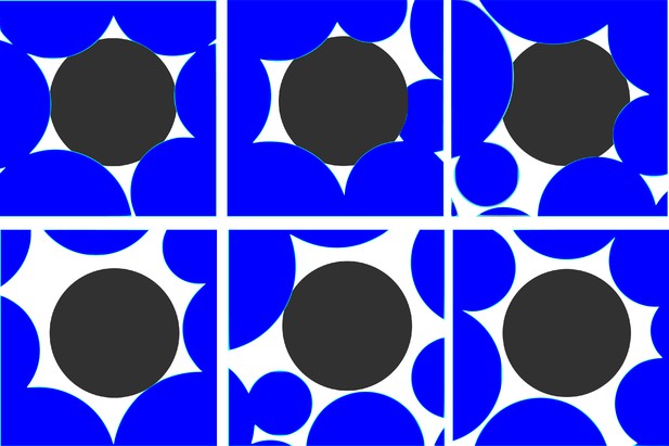
Dynamical rearrangement of jammed cells.

The changing local environment of a randomly selected cell (black) over time. Top panels: from left to right, $t = 9.41 τ_{α}, 10.01 τ_{α}$ , and $25.39 τ_{α}$ . The black-colored cell is completely jammed by other cells. Bottom panels: from left to right, $t = 10.97 τ_{α}, 25.44 τ_{α}$ , and $27.49 τ_{α}$ . Dynamical facilitation, resulting in collective rearrangement of the cells surrounding the black cell, enables it to move in the dynamically created free volume.

Appendix 7—figure 1

Download asset Open asset

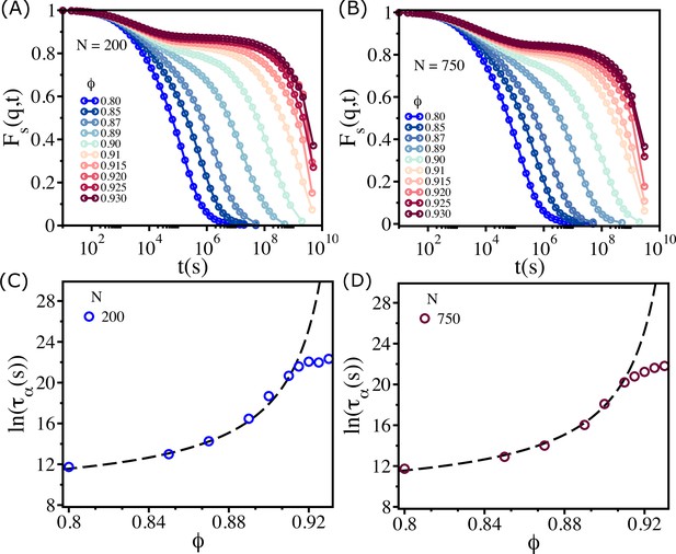
Finite size effects.

$F_{s} (q, t)$ for $N = 200$ (A) and $N = 750$ (B). Logarithm of $τ_{α}$ as a function of $ϕ$ for $N = 200$ (C) and for $N = 750$ (D). The dashed lines are the Vogel–Fulcher–Tammann (VFT) fits.

Appendix 8—figure 1

Download asset Open asset

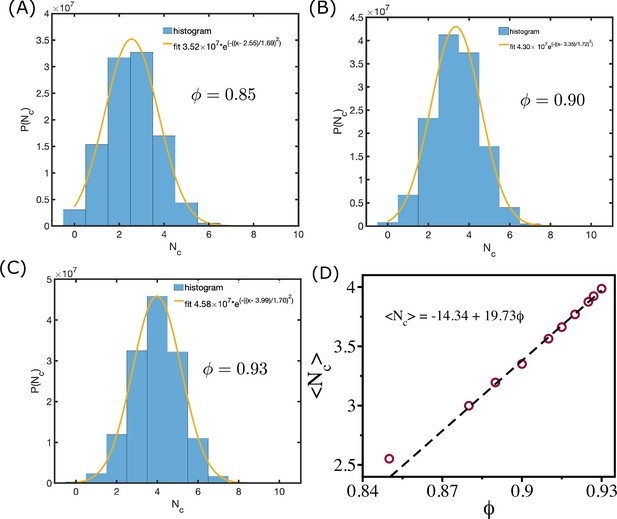
Mean coordination number and cell area fraction.

(A––C) shows the distribution of coordination number $P (N_{c})$ for $ϕ$ = 0.85, $0.90$ and $0.93$ , respectively. The orange lines are Gaussian fits to the histograms. (D) shows mean $⟨ N_{c} ⟩$ as a function of $ϕ$ . The dashed line shows the linear relationship between them.

Appendix 8—figure 2

Download asset Open asset

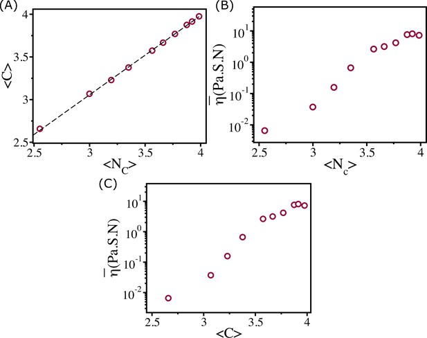
Viscosity and coordination number.

(A) shows $⟨ C ⟩$ as a function of $⟨ N_{c} ⟩$ . Clearly they are linearly related as shown by the dashed line. Viscosity $\bar{η}$ as a function of $⟨ N_{c} ⟩$ (B) and $⟨ C ⟩$ (C).

Appendix 9—figure 1

Download asset Open asset

Connectivity profile.

Connectivity maps for $ϕ = 0.80, 0.85, 0.89, 0.90, 0.92$ , and $0.93$ are shown in (A), (B), (C), (D), (E), and (F), respectively. For $ϕ \geq 0.89$ , there is a path that connects the cells in the entire sample. The percolation transition occurs over a very narrow range of $ϕ$ (roughly at $ϕ \approx 0.89$ ; orange map), which also coincides with the sharp increase in $η$ , thus linking equilibrium transition to geometric connectivity.

Videos

Video 1

Download asset

posterframe for video — Shows multiple rearrangements of smaller sized cells (blue and green cells) causes the big cells (yellow cells) to move in a highly jammed environment ( $ϕ = 0.92 > ϕ_{S}$ ).

Bright colors show the cell-cell overlap. Note that the overlap values are higher than those in lower area fractions. Free spaces (black background) are changing dynamically around a cell.

Video 2

Download asset

posterframe for video — Shows how a big cell (yellow) moves in the crowded environment $(ϕ = 0.90 (ϕ_{S}))$ .

Note that the smaller-sized cells (colored as deep blue) always move faster. Again, the multiple rearrangement causes the bigger cell to move substantially. The amount of overlap is smaller than that at $ϕ = 0.92$ .

Video 3

Download asset

posterframe for video — Shows the movements of cells at a low area fraction ( $ϕ = 0.85$ ).

Note that the smaller and bigger-sized cells are almost equally faster at lower area fractions ( $p h i = 0.85$ ) because of the huge available free areas.

Tables

Table 1

Parameters used in the simulation.

Parameters	Values	References
Timestep ( $Δ t$ )	$10 s$	This paper
Self-propulsion (µ)	$0.045 μ m / \sqrt{s}$	This paper
Friction coefficient ( $γ_{o}$ )	$0.1 k g / (μ m s)$	This paper
Mean cell elastic modulus ( $E_{i})$	$10^{- 3} M P a$	Galle et al., 2005; Malmi-Kakkada et al., 2018
Mean cell Poisson ratio ( $ν_{i}$ )	0.5	Schaller and Meyer-Hermann, 2005; Malmi-Kakkada et al., 2018

Additional files

MDAR checklist: https://cdn.elifesciences.org/articles/87966/elife-87966-mdarchecklist1-v1.pdf
Download elife-87966-mdarchecklist1-v1.pdf

Download links

A two-part list of links to download the article, or parts of the article, in various formats.

Downloads (link to download the article as PDF)

Article PDF

Open citations (links to open the citations from this article in various online reference manager services)

Mendeley

Cite this article (links to download the citations from this article in formats compatible with various reference manager tools)

Rajsekhar Das
Sumit Sinha
Xin Li
TR Kirkpatrick
D Thirumalai

(2024)

Free volume theory explains the unusual behavior of viscosity in a non-confluent tissue during morphogenesis

eLife 12:RP87966.

https://doi.org/10.7554/eLife.87966.4

Sign up for email alerts

Privacy notice