Drift of neural ensembles driven by slow fluctuations of intrinsic excitability
- Department of Bioengineering, Imperial College London, United Kingdom
- Department of Neuroscience, Icahn School of Medicine at Mount Sinai, United States
Figures
Figure 1 with 2 supplements
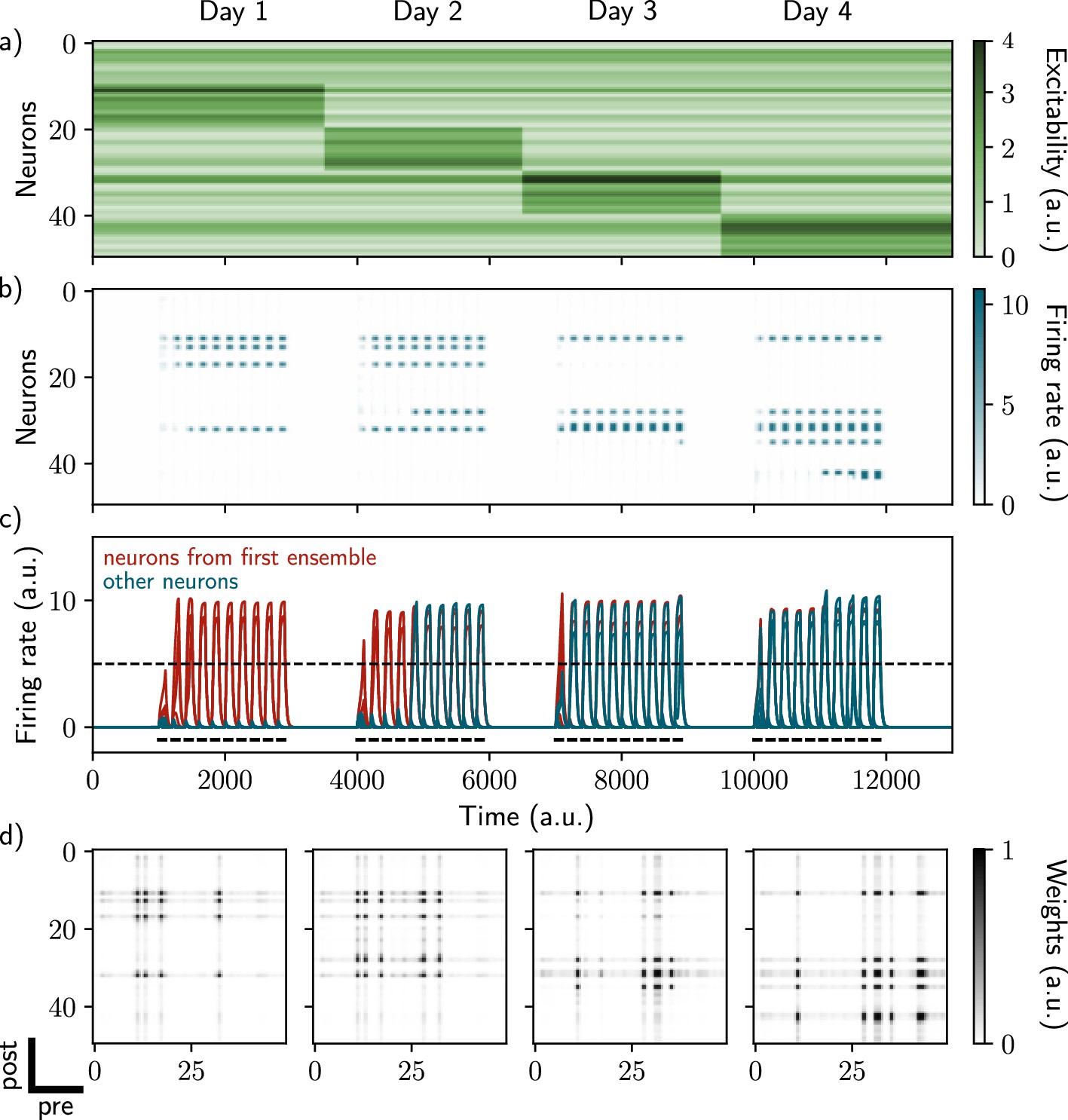
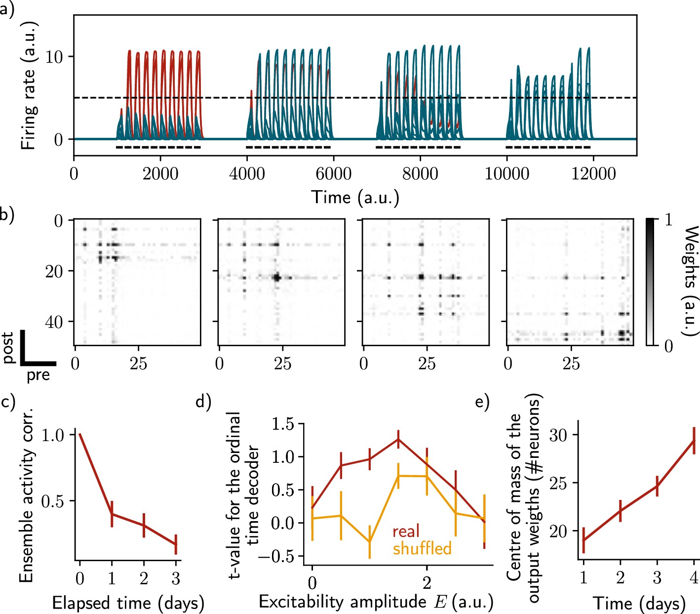
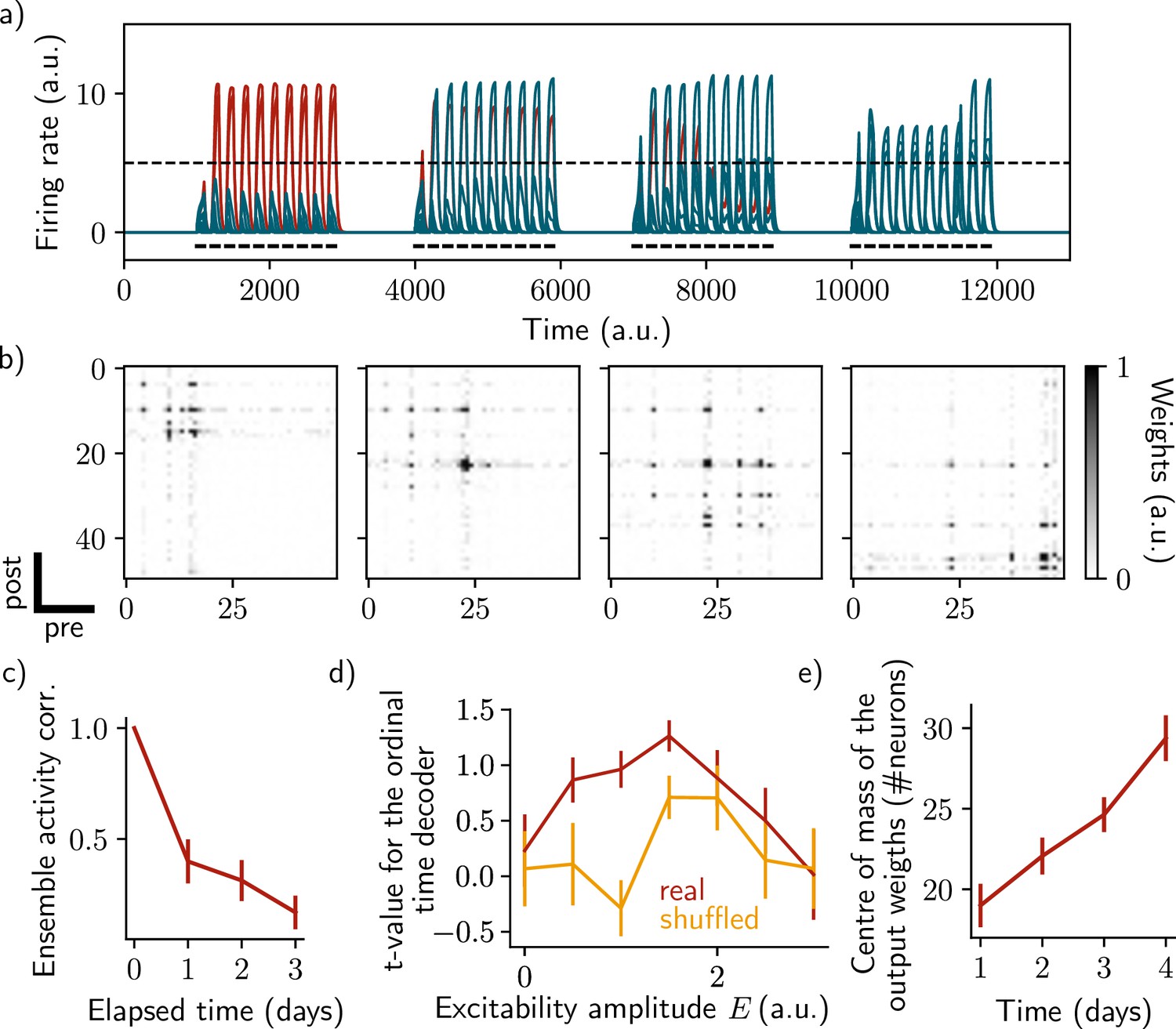
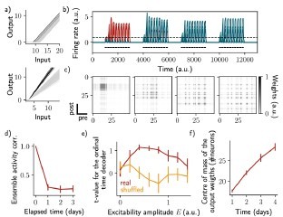
Excitability-induced drift of memory ensembles.
(a) Distribution of excitability for each neuron i, fluctuating over time. During each stimulation, a different pool of neurons has a high excitability (Methods). (b, c) Firing rates of the neurons across time. The red traces in panel (c) correspond to neurons belonging to the first assembly, namely that have a firing rate higher than the active threshold after the first stimulation. The black bars show the stimulation and the dashed line shows the active threshold. (d) Recurrent weights matrices after each of the four stimuli show the drifting assembly.
Figure 1—figure supplement 1
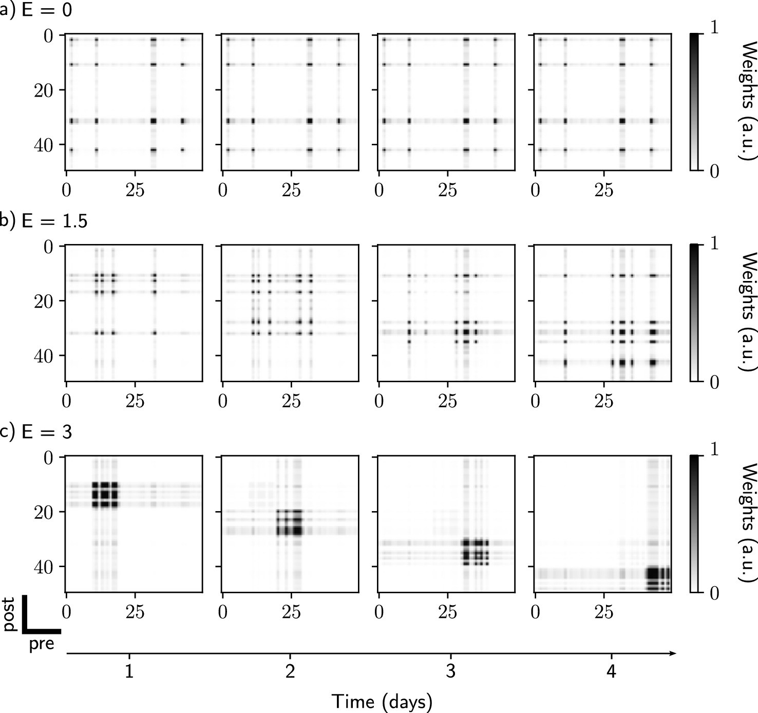
Comparison of drifting behavior for different values of excitability amplitude.
(a) , no drift. A neural assembly is initially formed during the first stimulation and later reactivated every subsequent day. (b) , partial drift. The ensemble is gradually modified during each new stimulation. (c) , full drift. Each new stimulation leads to formation of a new ensemble, containing neurons that have high excitability during this time.
Figure 1—figure supplement 2
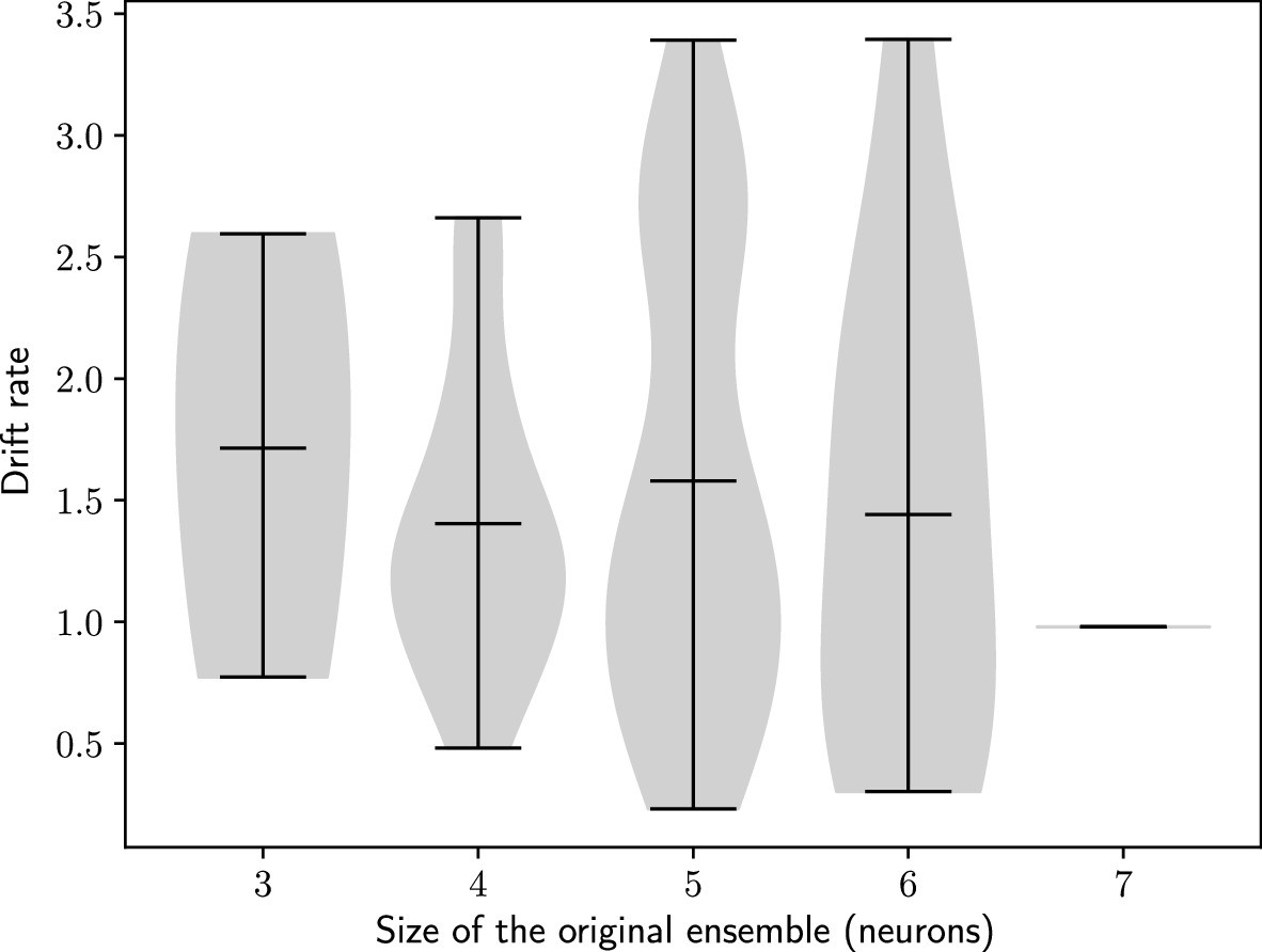
The rate of the drift does not depend on the size of the initial engram.
Drift rate against the size of the original engram. Bars show minimum, mean and maximum values. n=100 simulations.
Figure 2 with 4 supplements
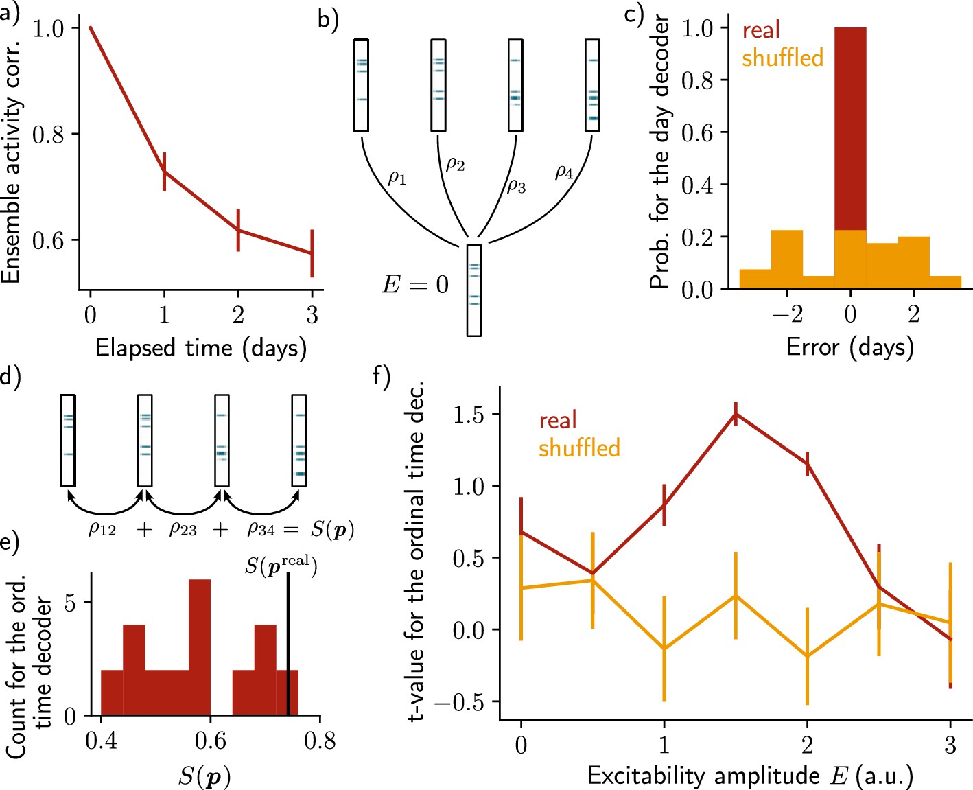
Neuronal activity is informative about the temporal structure of the reactivations.
(a) Correlation of the patterns of activity between the first day and every other days, for n=10 simulations. Data are shown as mean ± s.e.m. (b) Schema of the day decoder. The day decoder maximises correlation between the patterns of each day with the pattern from the simulation with no increase in excitability. (c) Results of the day decoder for the real data (red) and the shuffled data (orange). Shuffled data consist of the same activity pattern for which the label of each cell for every seed has been shuffled randomly. For each simulation, the error is measured for each day as the difference between the decoded and the real day. Data are shown for n=10 simulations and for each of the 4 days. (d) Schema of the ordinal time decoder. This decoder output the permutation that maximises the sum of the correlations of the patterns for each pairs of days. (e) Distribution of the value for each permutation of days . The value for the real permutation is shown in black. (f) Student’s test t-value for n=10 simulations, for the real (red) and shuffled (orange) data and for different amplitudes of excitability . Data are shown as mean ± s.e.m. for n=10 simulations.
Figure 2—figure supplement 1
Sparse recurrent connectivity shows similar drifting behavior as all-to-all connectivity.
The same simulation protocol as Figure 1 was used while the recurrent weights matrix was made 50% sparse (Methods). (a) Firing rates of the neurons across time. The red traces correspond to neurons belonging to the first assembly, namely that have a firing rate higher than the active threshold after the first stimulation. The black bars show the stimulation and the dashed line shows the active threshold. (b) Recurrent weights matrices after each of the four stimuli show the drifting assembly. (c) Correlation of the patterns of activity between the first day and every other days. (d) Student’s test t-value of the ordinal time decoder, for the real (red) and shuffled (orange) data and for different amplitudes of excitability . (e) Center of mass of the distribution of the output weights (Methods) across days. (c–e) Data are shown as mean ± s.e.m. for n=10 simulations.
Figure 2—figure supplement 2
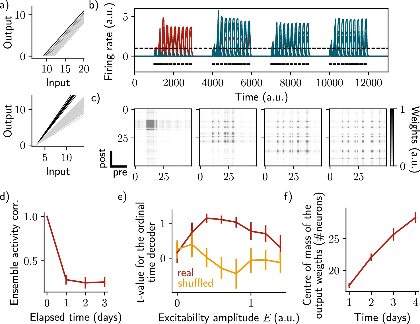
Change of excitability as a variable slope of the input-output function shows similar drifting behavior as considering a change in the threshold.
The same simulation protocol as Figure 1 was used while the excitability changes were modeled as a change in the slope of the activation function (Methods). (a) Schema showing two different ways of defining excitability, as a threshold (top) or slope (bottom) of the activation function. Each line shows one neuron and darker lines correspond to neurons with increased excitability. (b) Firing rates of the neurons across time. The red traces correspond to neurons belonging to the first assembly, namely that have a firing rate higher than the active threshold after the first stimulation. The black bars show the stimulation and the dashed line shows the active threshold. (c) Recurrent weights matrices after each of the four stimuli show the drifting assembly. (d) Correlation of the patterns of activity between the first day and every other days. (e) Student’s test t-value of the ordinal time decoder, for the real (red) and shuffled (orange) data and for different amplitudes of excitability . (f) Center of mass of the distribution of the output weights (Methods) across days. (d-f) Data are shown as mean ± s.e.m. for n=10 simulations.
Figure 2—figure supplement 3

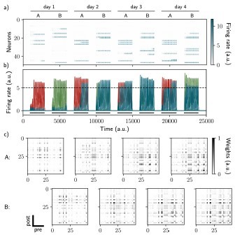
Two distinct ensembles can be encoded and drift independently.
(a, b) Firing rates of the neurons across time. The red traces in panel (b) correspond to neurons belonging to the first assembly and the green traces to the second assembly on the first day. They correspond to neurons having a firing rate higher than the active threshold after the first stimulation of each assembly. The black bars show the stimulation and the dashed line shows the active threshold. (c) Recurrent weights matrices after each of the eight stimuli showing the drifting of the first (top) and second (bottom) assembly.
Figure 2—figure supplement 4
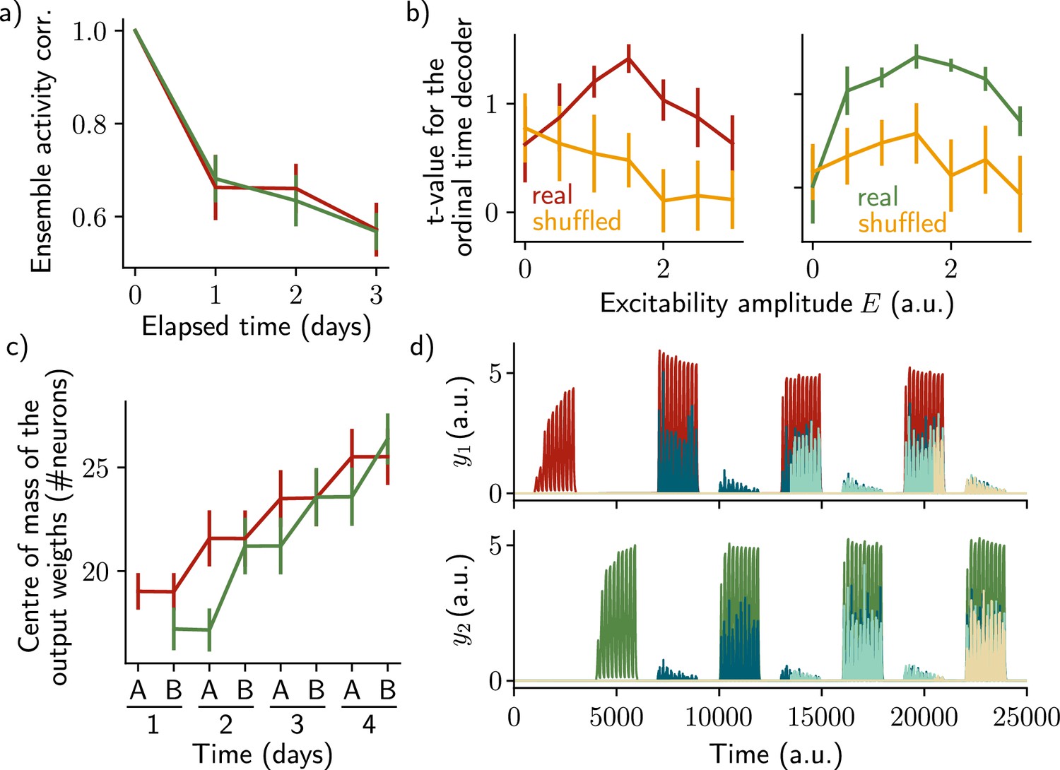
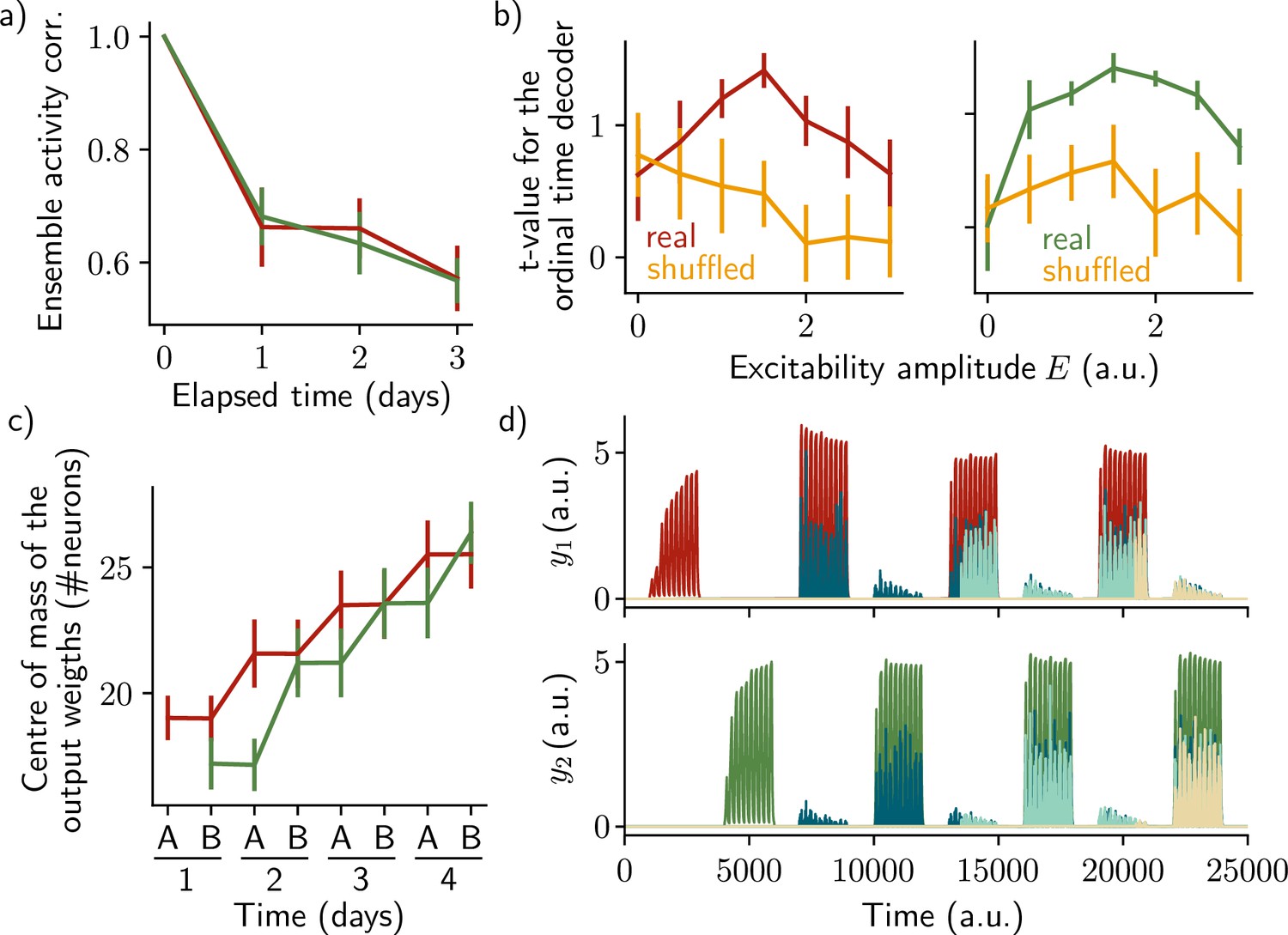
The two ensembles are informative about their temporal history and can be decoded using two output neurons.
(a) Correlation of the patterns of activity between the first day and every other days, for the first assembly (red) and the second assembly (green). (b) Student’s test t-value of the ordinal time decoder, for the first (red, left) and second ensemble (green, right) for different amplitudes of excitability . Shuffled data are shown in orange. (c) Center of mass of the distribution of the output weights (Methods) across days for the first (, red) and second (, green) ensemble. (a–c) Data are shown as mean ± s.e.m. for n=10 simulations. (d) Output neurons firing rate across time for the first ensemble (, top) and the second ensemble (, bottom). The red and green traces correspond to the real output. The dark blue, light blue and yellow traces correspond to the cases where the output weights were randomly shuffled for every time points after presentation of the first, second and third stimulus, respectively.
Figure 3 with 1 supplement
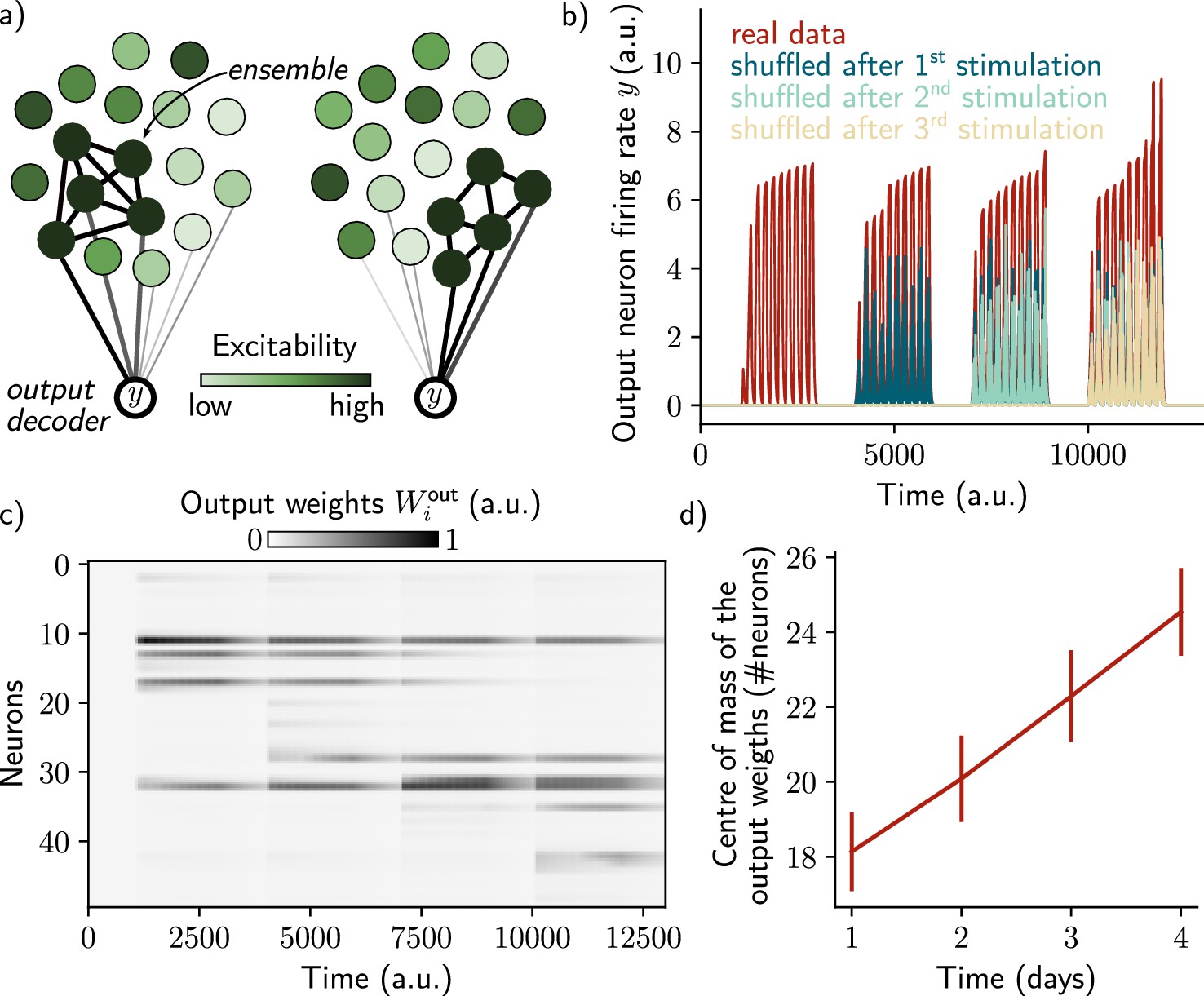
A single output neuron can track the memory ensemble through Hebbian plasticity.
(a) Conceptual architecture of the network: the read-out neuron in red ‘tracks’ the ensemble by decreasing synapses linked to the previous ensemble and increasing new ones to linked to the new assembly. (b) Output neuron’s firing rate across time. The red trace corresponds to the real output. The dark blue, light blue and yellow traces correspond to the cases where the output weights were randomly shuffled for every time points after presentation of the first, second and third stimulus, respectively. (c) Output weights for each neuron across time. (d) Center of mass of the distribution of the output weights (Methods) across days. The output weights are centered around the neurons that belong to the assembly at each day. Data are shown as mean ± s.e.m. for n=10 simulations.
Figure 3—figure supplement 1
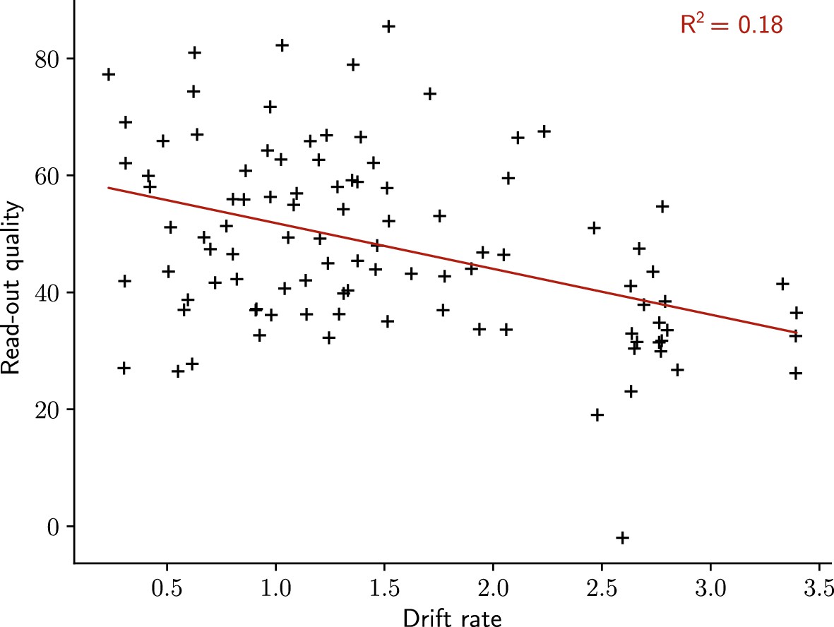
The quality of the read-out decreases with the rate of the drift.
Read-out quality computed on the firing rate of the output neuron against the rate of the drift (Methods). Each dot shows one simulation. n=100 simulations.
Author response image 1

The rate of the drift does not depend on the size of the engram.
Drift rate against the size of the original engram. Each dot shows one simulation (Methods). n = 100 simulations.
Author response image 2
Sparse recurrent connectivity shows similar drifting behavior as all-to-all connectivity.
The same simulation protocol as Fig. 1 was used while the recurrent weights matrix was made 50% sparse (Methods). (a) Firing rates of the neurons across time. The red traces correspond to neurons belonging to the first assembly, namely that have a firing rate higher than the active threshold after the first stimulation. The black bars show the stimulation and the dashed line shows the active threshold. (b) Recurrent weights matrices after each of the four stimuli show the drifting assembly. (c) Correlation of the patterns of activity between the first day and every other days. (d) Student's test t-value of the ordinal time decoder, for the real (red) and shuffled (orange) data and for different amplitudes of excitability E. (e) Center of mass of the distribution of the output weights (Methods) across days. (c-e) Data are shown as mean ± s.e.m. for n = 10 simulations.
Author response image 3
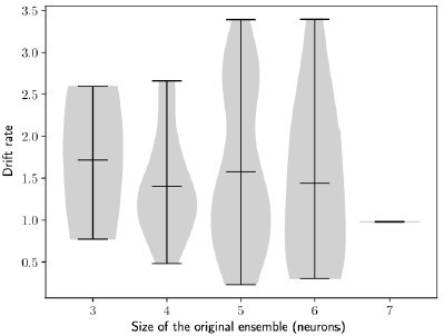
The rate of the drift does not depend on the size of the engram.
Drift rate against the size of the original engram. Each dot shows one simulation (Methods). n = 100 simulations.
Author response image 4

The quality of the read-out decreases with the rate of the drift.
Read-out quality computed on the firing rate of the output neuron against the rate of the drift (Methods). Each dot shows one simulation. n = 100 simulations.
Author response image 5
Change of excitability as a variable slope of the input-output function shows similar drifting behavior as considering a change in the threshold.
The same simulation protocol as Fig. 1 was used while the excitability changes were modeled as a change in the activation function slope (Methods). (a) Schema showing two different ways of defining excitability, as a threshold (top) or slope (bottom) of the activation function. Each line shows one neuron and darker lines correspond to neurons with increased excitability. (b) Firing rates of the neurons across time. The red traces correspond to neurons belonging to the first assembly, namely that have a firing rate higher than the active threshold after the first stimulation. The black bars show the stimulation and the dashed line shows the active threshold. (c) Recurrent weights matrices after each of the four stimuli show the drifting assembly. (d) Correlation of the patterns of activity between the first day and every other days. (e) Student's test t-value of the ordinal time decoder, for the real (red) and shuffled (orange) data and for different amplitudes of excitability E. (f) Center of mass of the distribution of the output weights (Methods) across days. (d-f) Data are shown as mean ± s.e.m. for n = 10 simulations.
Author response image 6
Two distinct ensembles can be encoded and drift independently.
a) and b) Firing rates of the neurons across time. The red traces in panel b) correspond to neurons belonging to the first assembly and the green traces to the second assembly on the first day. They correspond to neurons having a firing rate higher than the active threshold after the first stimulation of each assembly. The black bars show the stimulation and the dashed line shows the active threshold. c) Recurrent weights matrices after each of the eight stimuli showing the drifting of the first (top) and second (bottom) assembly.
Author response image 7
The two ensembles are informative about their temporal history and can be decoded using two output neurons.
a) Correlation of the patterns of activity between the first day and every other days, for the first assembly (red) and the second assembly (green). b) Student's test t-value of the ordinal time decoder, for the first (red, left) and second ensemble (green, right) for different amplitudes of excitability E. Shuffled data are shown in orange. c) Center of mass of the distribution of the output weights (Methods) across days for the first (w?ut , red) and second (W20L't , green) ensemble. a-c) Data are shown as mean ± s.e.m. for n = 10 simulations. d) Output neurons firing rate across time for the first ensemble (Yl, top) and the second ensemble (h, bottom). The red and green traces correspond to the real output. The dark blue, light blue and yellow traces correspond to the cases where the output weights were randomly shuffled for every time points after presentation of the first, second and third stimulus, respectively.
Additional files
Download links
A two-part list of links to download the article, or parts of the article, in various formats.
Downloads (link to download the article as PDF)
Open citations (links to open the citations from this article in various online reference manager services)
Cite this article (links to download the citations from this article in formats compatible with various reference manager tools)
Drift of neural ensembles driven by slow fluctuations of intrinsic excitability
eLife 12:RP88053.
https://doi.org/10.7554/eLife.88053.3


