Passive exposure to task-relevant stimuli enhances categorization learning
- Institute of Neuroscience, University of Oregon, United States
- Department of Linguistics, University of Oregon, United States
Figures
Figure 1
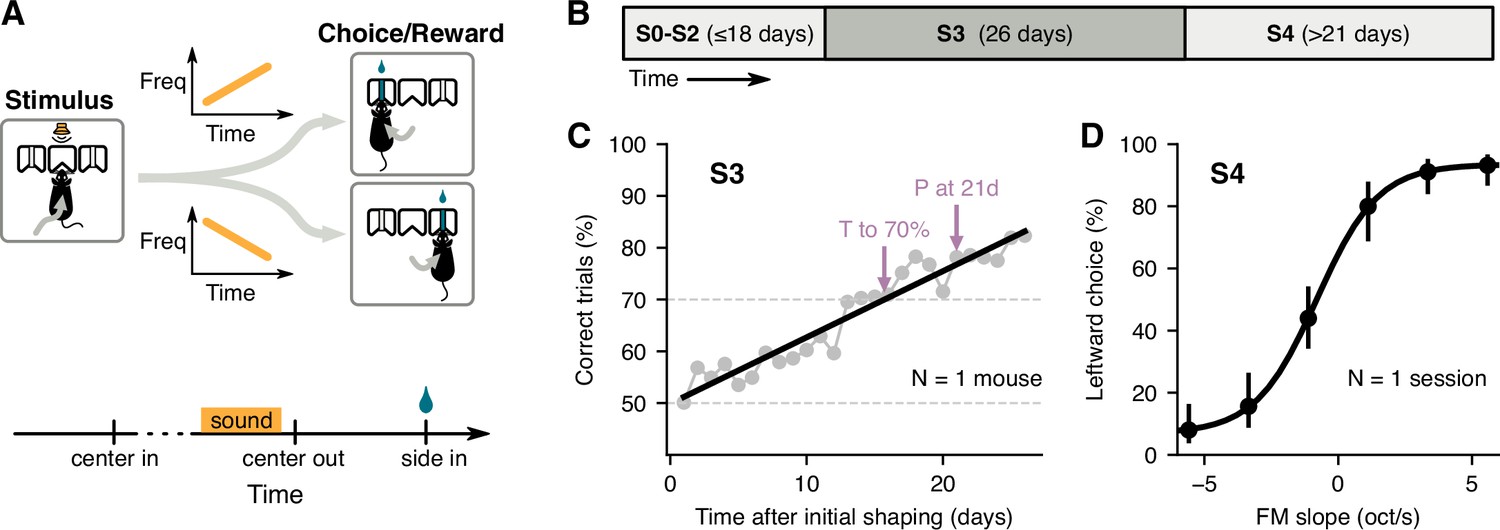
Two-alternative choice sound-categorization task for mice.
(A) Mice initiated a trial by poking their nose into the center port of a three-port chamber, triggering the presentation of a frequency-modulated (FM) sound. To obtain reward, animals had to choose the correct side port according to the slope of the frequency modulation (left for positive slopes, right for negative slopes). (B) Training schedule: mice underwent several shaping stages (S0–S2) before learning the full task; the main learning stage (stage S3) used only the highest and lowest FM slopes; psychometric performance was evaluated using 6 different FM slopes (stage S4). (C) Daily performance for one mouse during S3. Arrows indicate estimates of the time to reach 70% correct and the performance at 21 days given a linear fit (black line). (D) Average leftward choices for each FM slope during one session of S4 for the mouse in C. Error bars indicate 95% confidence intervals.
Figure 2
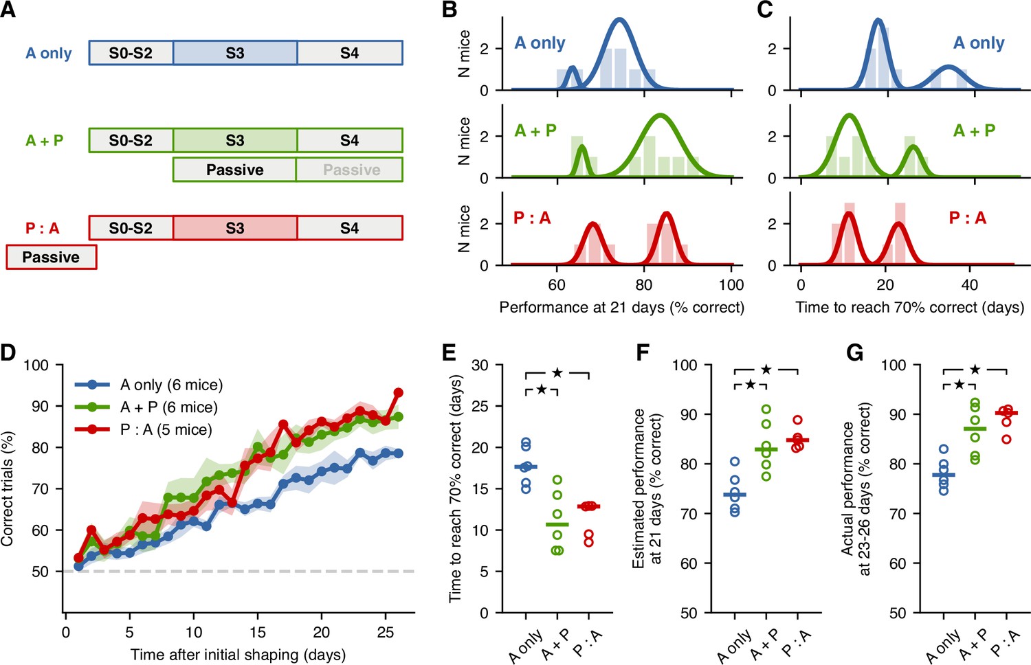
Passive exposure to sounds improves learning speed.
(A) Training schedule for each mouse cohort: A-only mice received no passive exposure; A + P mice received passiveexposure sessions during stage S3; P:A mice received a similar number of passive-exposure sessions before S2. (B) Distributions of performance at 21 days of S3 given estimates from linear fits to the learning curve for each mouse from each cohort. Solid lines represent the results from a Gaussian mixture model with two components, separating ‘fast’ from ‘slow’ learners. (C) Distributions of times to reach 70% correct given estimates from linear fits. (D) Average learning curves across fast learners from each cohort. Shading represent the standard error of the mean across mice. (E) Estimates of the time to reach 70% for fast learners from each group. Each circle is one mouse. Horizontal bar represents the median. (F) Estimates of the performance at 21 days for fast learners from each group. (G) Actual performance averaged across the last 4 days of S3 for fast learners from each group. Stars indicate .
Figure 3
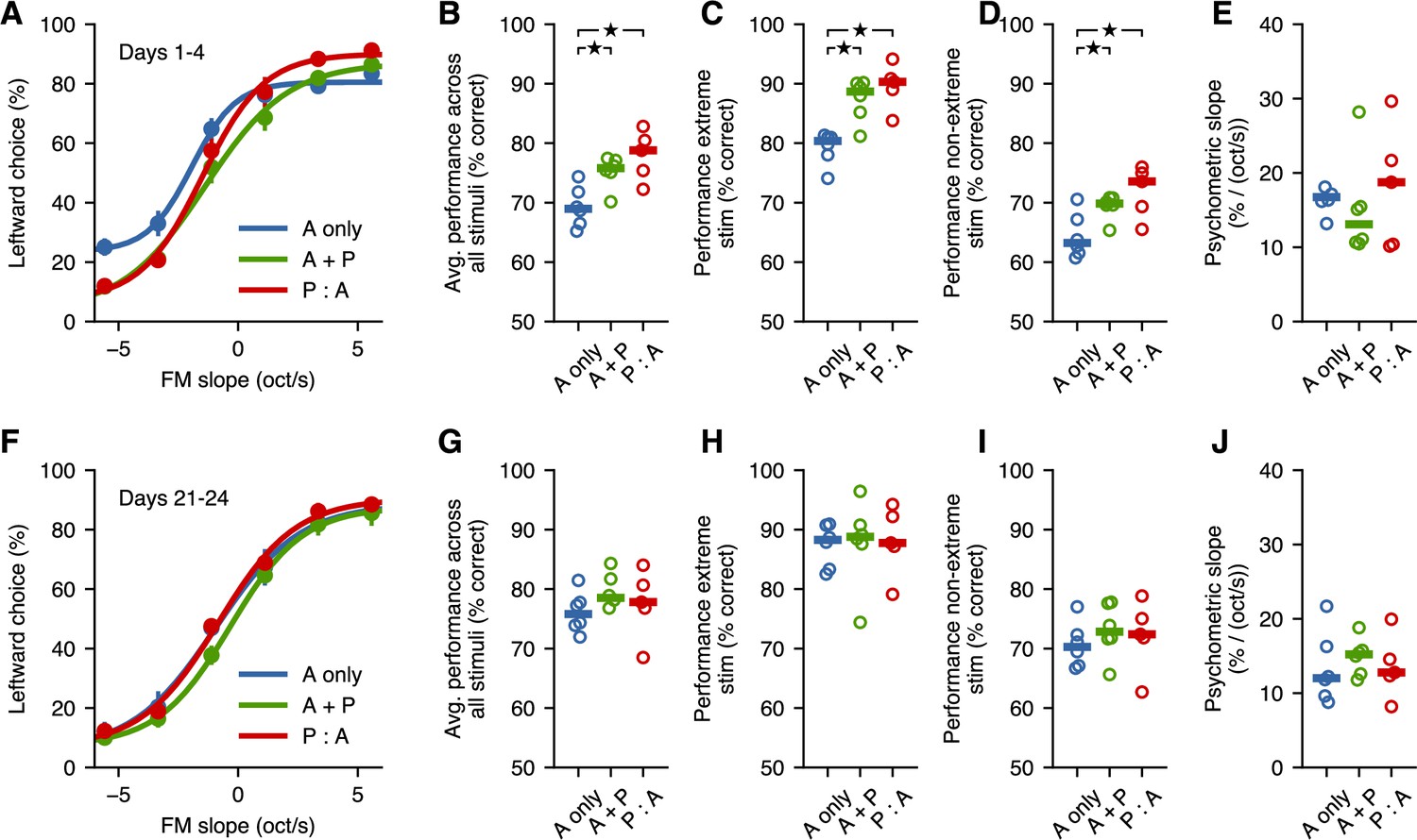
Passive exposure improves categorization of intermediate stimuli.
(A) Average psychometric performance for the first 4 days of stage S4 across fast learners from each group. Error bars show the standard error of the mean across mice. (B) Performance averaged across all stimuli is better for mice with passive exposure. Horizontal lines indicate median across mice. (C) Performance for extreme stimuli (included in S3) is better for mice with passive exposure. (D) Performance for intermediate stimuli (which were not used in the task before S4) is better for mice with passive exposure. (E) Psychometric slope is not different across groups. (F–J) All groups achieve similar levels of performance after 3 weeks of additional training. Stars indicate .
Figure 4
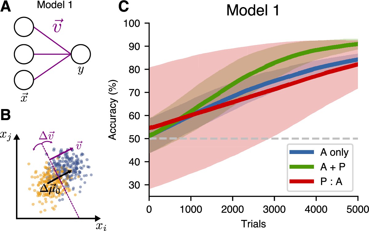
A single-layer model (Model 1) does not benefit from passive pre-exposure.
(A) Network architecture for the one-layer model. (B) The network is trained to find a hyperplane orthogonal to the decoding direction . (C) Learning performance for different training schedules. Curves show mean accuracy for network realizations, and shading shows standard deviation.
Figure 5
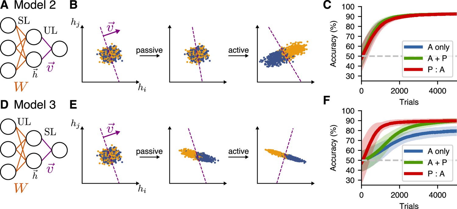
Passive-exposure benefits learning in a two-layer model with unsupervised learning in the first layer.
(A) Network architecture for Model 2, which has supervised learning (SL) at the input layer, and unsupervised learning (UL) at the readout. (B) Learning dynamics of the hidden-layer representation of this model for the P:A schedule. (C) Learning performance for different training schedules for Model 2. Curves show mean accuracy for network realizations, and shading shows standard deviation. (D–F) Model 3, which has unsupervised learning (UL) at the input layer, and supervised learning (SL) at the readout.
Figure 6
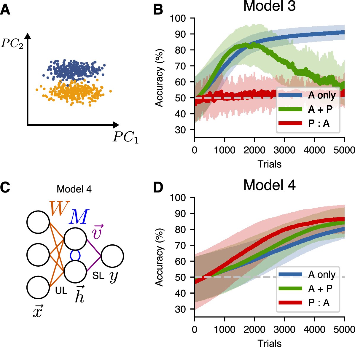
An alternative unsupervised learning rule can be used to learn hidden representations of higher principal components.
(A) A non-isotropic input distribution in which the coding dimension does not align with the direction of highest variance. (B) Learning performance for Model 3 on the non-isotropic input distribution. Curves show mean accuracy for network realizations, and shading shows standard deviation. (C) Network architecture for a two-layer model (Model 4) that uses the similarity matching algorithm for the input weights and supervised learning at the readout. (D) Learning performance for Model 4 on the non-isotropic input distributions.
Figure 7
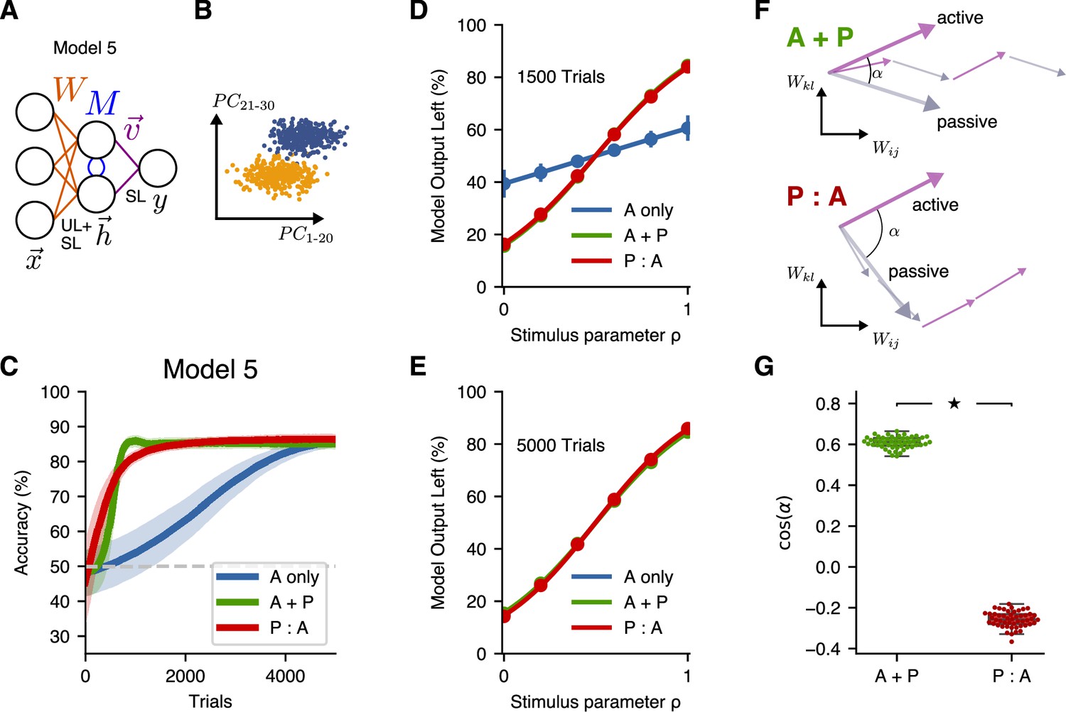
A more-general two-layer model accounts for similar benefits of A + P and P:A training schedules.
(A) Schematic illustration of Model 5, which combines supervised and unsupervised learning at the input layer of weights. (B) Input distribution, in which the decoding direction is not aligned with any particular principal component. (C) Learning performance of Model 5. Curves show mean accuracy for $ network realizations, and shading shows standard deviation. (D) Psychometric curves showing classification performance for all stimuli after 1500 trials, where the stimulus parameter linearly interpolates between the two extreme stimulus values. (E) Psychometric curves showing classification performance after 5000 trials. (F) Schematic illustration of the angle between the summed weight updates during active training and passive exposure for A + P (top) and P:A (bottom) learners. (G) The alignment of active and passive weight updates for networks trained with either the A + P or P:A schedule after 1500 trials (star indicates , Wilcoxon rank-sum test; box percentiles are 25/75).
Tables
Table 1
Hyperparameters used for shown results.
| Model 1 | Model 2 | Model 3 | Model 4 | Model 5 | |
|---|---|---|---|---|---|
| 1·10−4 | 5·10−2 | – | – | 1·10−5 | |
| 2.4 | 1 | – | – | 1 | |
| 2·10−4 | – | 1·10−2 | 3·10−3 | 2·10−3 | |
| 5·10−2 | – | 2·10−2 | 3·10−2 | 5·10−2 | |
| – | – | 2·10−5 | 8·10−6 | 6·10−5 | |
| – | – | 1 | 1 | 4 | |
| – | 1·10−3 | – | – | 1·10−4 | |
| – | 1.10−3 | – | – | 1·10−3 |
Additional files
Download links
A two-part list of links to download the article, or parts of the article, in various formats.
Downloads (link to download the article as PDF)
Open citations (links to open the citations from this article in various online reference manager services)
Cite this article (links to download the citations from this article in formats compatible with various reference manager tools)
Passive exposure to task-relevant stimuli enhances categorization learning
eLife 12:RP88406.
https://doi.org/10.7554/eLife.88406.3


