Figures and data in Tools and methods for high-throughput single-cell imaging with the mother machine

Figures
Tables
Additional files

7 figures, 4 tables and 1 additional file

Figures

Figure 1 with 1 supplement

Download asset Open asset

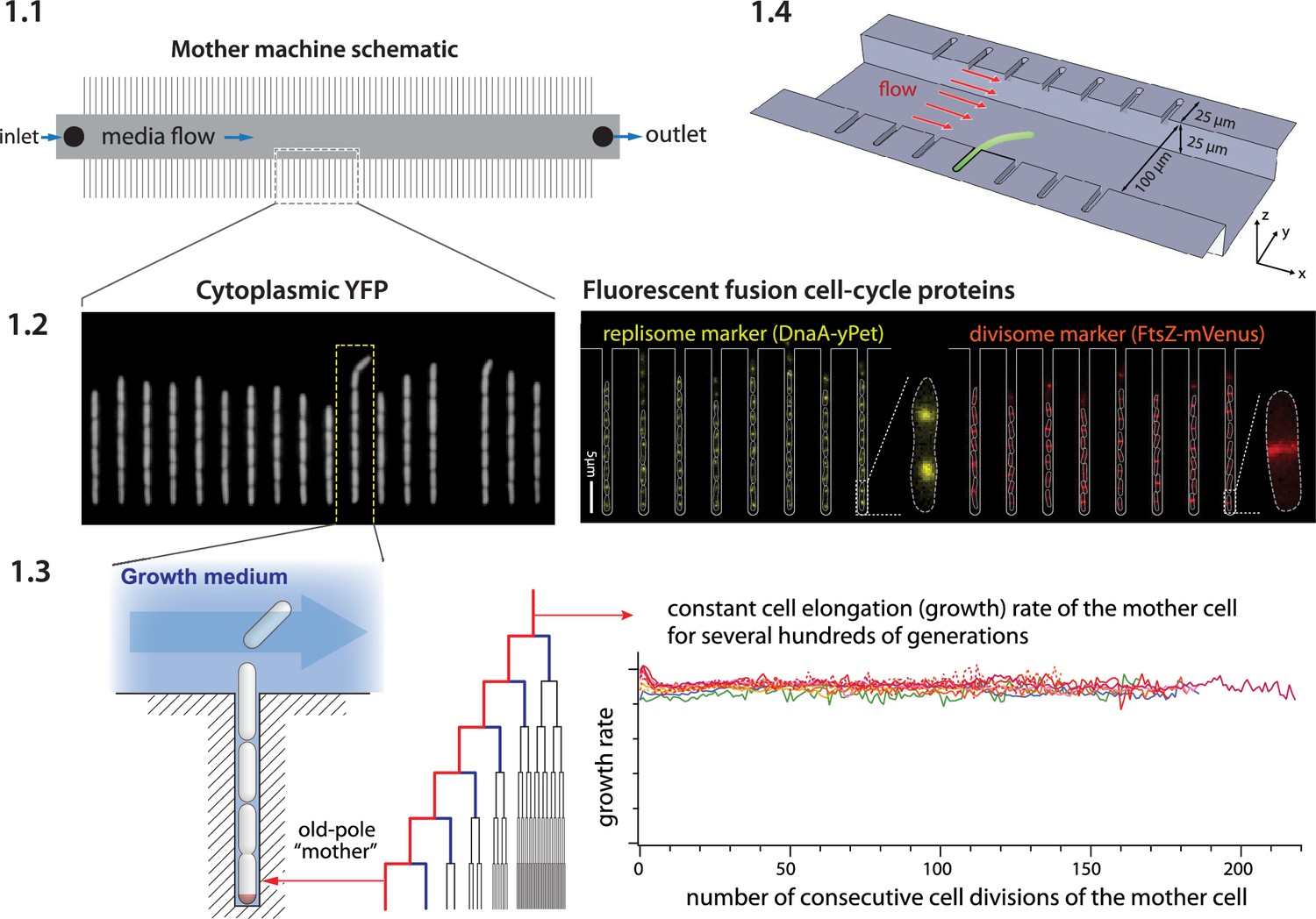
Mother machine workflow, schematic, and applications.

(**1.1**) Mother machine schematic. Growth channels flank a central flow cell that supplies fresh media and whisks away daughter cells. In a typical experiment, numerous fields of view (FOVs) are imaged for several hours. (**1.2**) Fluorescence images of *E. coli* strains expressing cytoplasmic YFP (Wang et al., 2010) (left) and markers for the replisome protein DnaN and division protein FtsZ (right) (Si et al., 2019). (**1.3**) The mother machine setup allows long-term monitoring of the old-pole mother cell lineage (Wang et al., 2010) and has other versatile applications, including (**1.4**) the study of the mechanical properties of bacterial cells by applying controlled Stokes forces (Amir et al., 2014).

Figure 1—figure supplement 1

Download asset Open asset

Inexpensive fabrication of cell loader with 3D printing.

An inexpensive device for loading cells into the mother machine. The construction involves 3D printing a custom holder/rotor for a 50-mm WillCo dish, on which a mother machine is attached. The holder is printed in three parts (two blades and a central base) to account for 3D printers with small printing areas. This piece is then assembled and secured to a Honeywell fan from which the original blade has been removed. CAD files and details of the fan centrifuge construction are available at Thiermann, 2023.

Box 1—figure 1

Download asset Open asset

Duplication and distribution of mother machine devices with epoxy molds.

Figure 2

Download asset Open asset

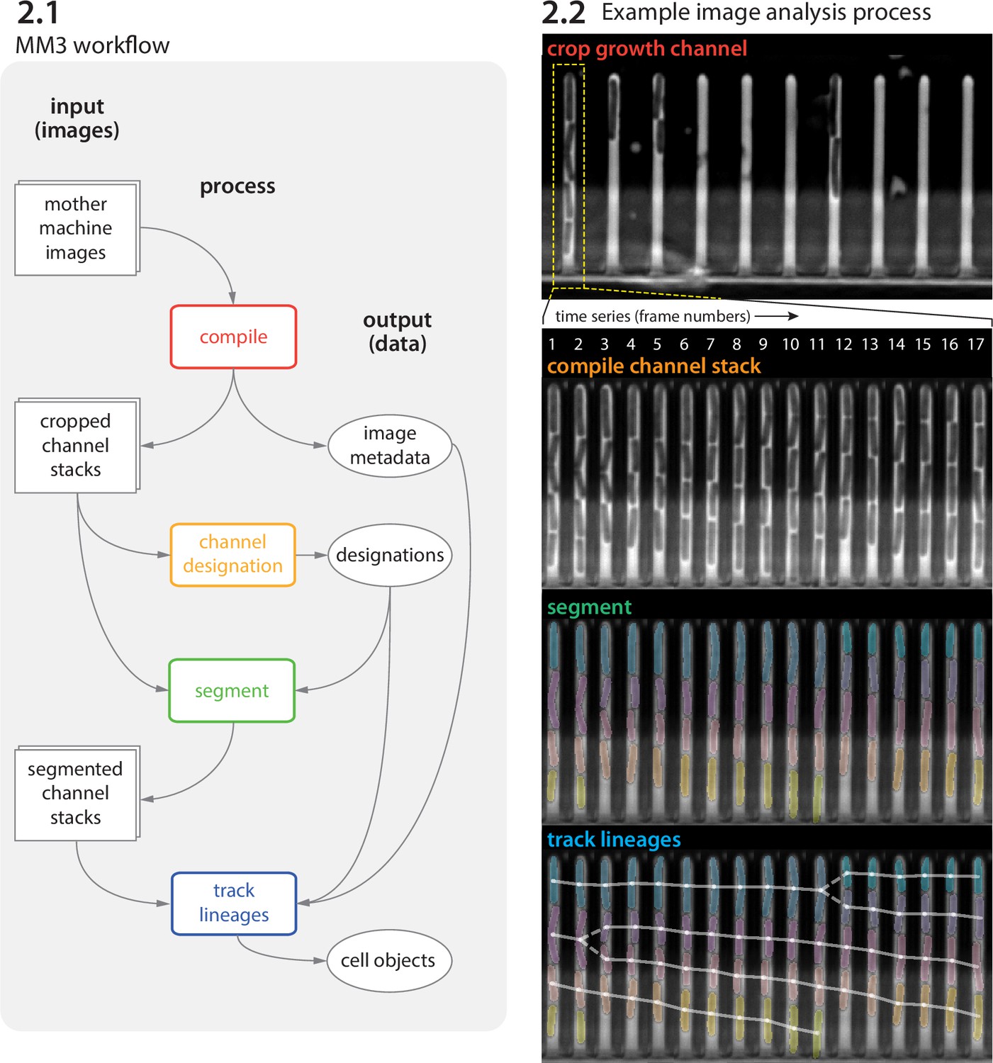
MM3 workflow and example images.

(**2.1**) The MM3 image analysis pipeline takes raw mother machine images and produces cell objects. Processes (rounded rectangles) are modular; multiple methods are provided for each. (**2.2**) Example images from the processing of one growth channel in a single field of view (FOV). The growth channel is first identified, cropped, and compiled in time. All cells are segmented (colored regions). Lineages are tracked by linking segments in time to determine growth and division (solid and dashed lines, respectively), creating cell objects.

Figure 3

Download asset Open asset

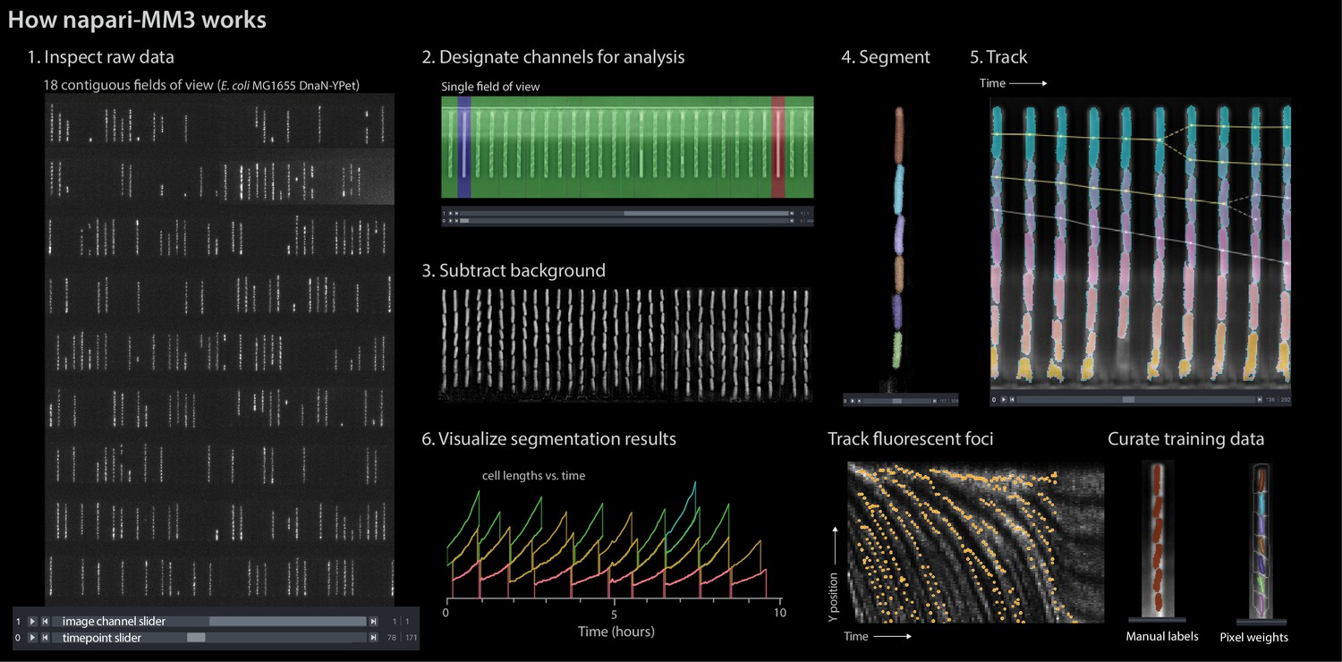
napari-MM3 interface.

The napari viewer enables interactive analysis of mother machine data with real-time feedback and fast debugging. Raw data shown is from MG1655 background *E coli* expressing the fluorescence protein YPet fused to the replisome protein DnaN (Si et al., 2019).

Box 2—figure 1

Download asset Open asset

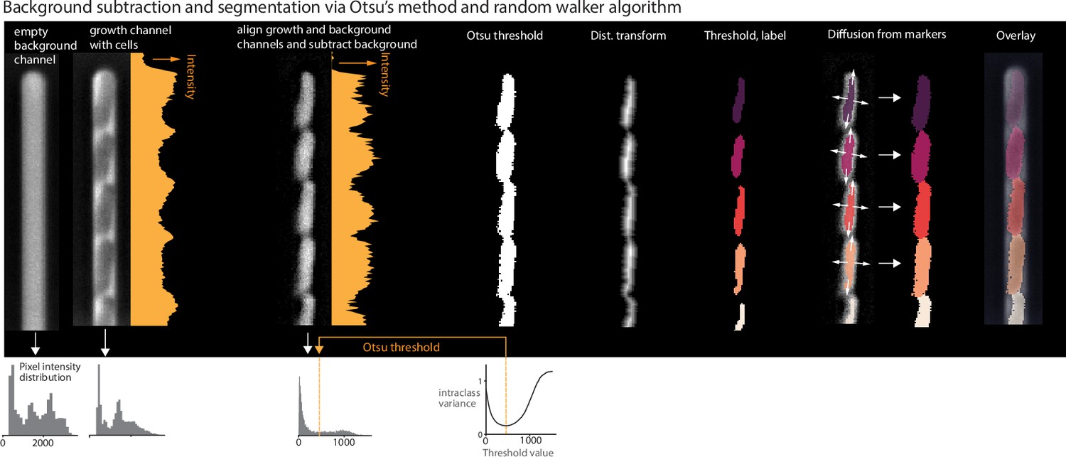
Background subtraction and segmentation via Otsu's method and random walker algorithm.

Figure 4 with 1 supplement

Download asset Open asset

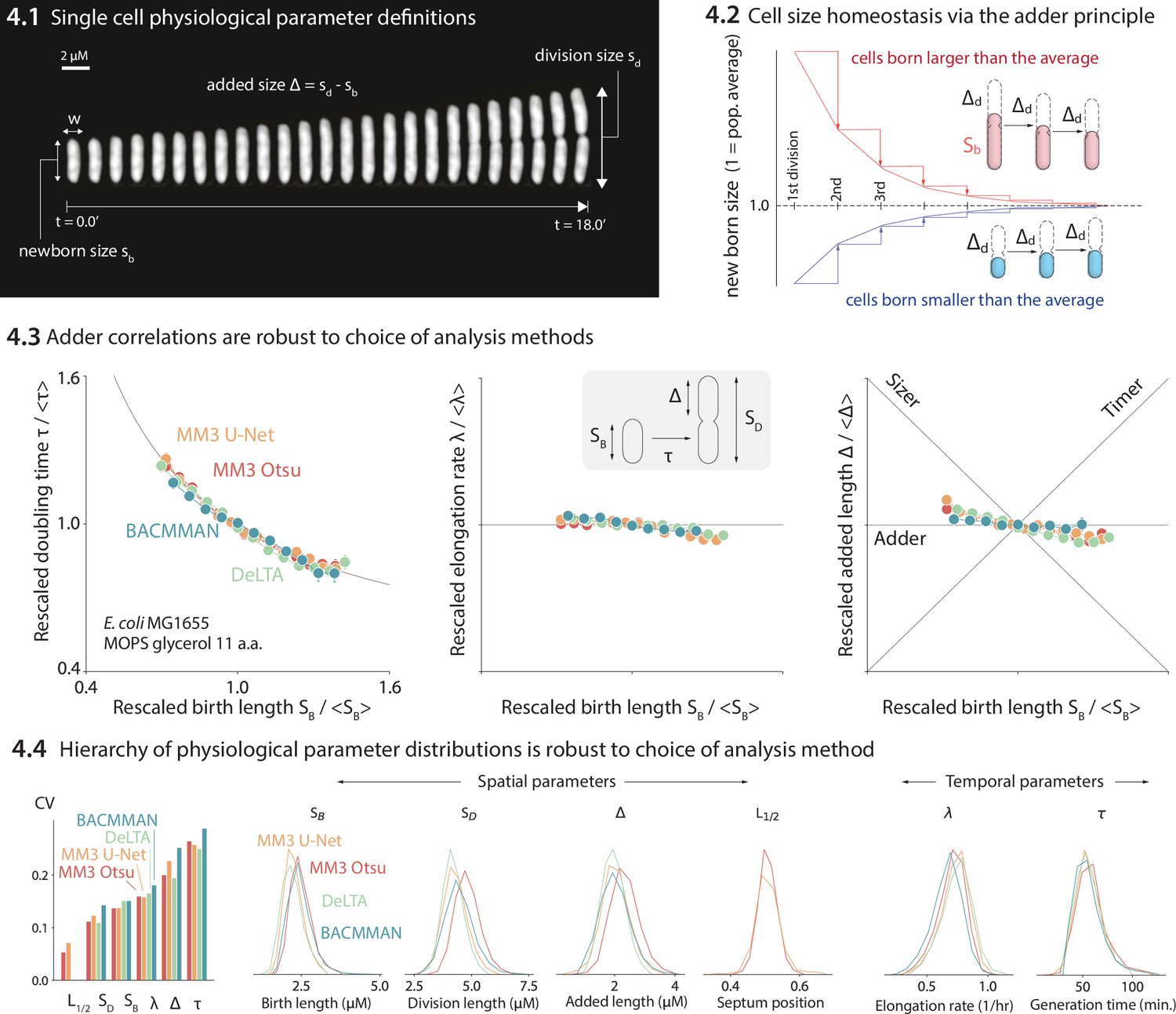
Comparison of various image analysis approaches.

(**4.1**) A time series of a typical cell growing in a nutrient-rich medium. The birth size, division size, and added size are indicated. (**4.2**) The adder principle ensures cell size homeostasis via passive convergence of cell size to the population mean. (**4.3**) We analyzed multiple datasets from our lab using MM3, DeLTA, and BACMMAN, and obtained robust correlations between birth length, doubling time, elongation rate, and added length. Representative results from one dataset (Si et al., 2019) for MG1655 background *E. coli* grown in MOPS glycerol + 11 amino acids are shown, with 9000–13,000 cells analyzed depending on the method. Error bars indicate standard error of the mean (note the standard error is smaller than marker size in most cases). (**4.4**) Distributions of key physiological parameters are independent of the analysis methods. The data and code used to generate this figure are available at Thiermann, 2024a.

Figure 4—figure supplement 1

Download asset Open asset

Old-pole aging phenotype is strain specific.

Cells imaged with fluorescence often show signs of aging in the old-pole ‘mother’ cell. For instance, in the dataset analyzed in Figure 4 (*E. coli* MG1655 with the fluorescent protein YPet fused to DnaN), we observed systematic differences in cell elongation rate and size between the old-pole cell at the end of the growth channel and its sisters, which inherit the new pole (top center). However, this asymmetry is not universal. Using napari-MM3’s Otsu segmentation method, we re-analyzed previously published data obtained without fluorescence illumination (Taheri-Araghi et al., 2015a), and found that the old- and new-pole cell elongation rates varied only on the order of 1% (lower center), while in the dataset obtained under fluorescence imaging, the old-pole mother cells grow 7–10% slower than the new-pole cells. Cells born third or fourth from the closed end of the channel also grow slower than the old-pole mother (right). The asymmetry in growth rate between old- and new-pole cells persists across time (right, inset). These results are consistent with a previous survey (Rang et al., 2012), which found that most evidence for aging in *E. coli* comes from studies utilizing fluorescent proteins for visualization.

Figure 5 with 1 supplement

Download asset Open asset

Effect of systematic deviation in segmentation output from different methods.

(**5.1**) Otsu/random walker and U-Net segmentation masks. The classical method systematically yields masks that are 5–10% larger than the other methods. (**5.2**) We confirmed that this discrepancy occurs consistently across the cell cycle. (**5.3**) We trained the Omnipose model on masks generated by either napari-MM3-Otsu or napari-MM3-U-Net separately. (**5.4**) The systematic discrepancy in the training data masks propagated to the output of the trained models.

Figure 5—figure supplement 1

Download asset Open asset

Evaluating segmentation output of napari-MM3 Otsu and U-Net methods.

To evaluate the quality of the segmentation masks generated by MM3’s Otsu and U-Net segmentation methods, we computed the Jaccard index (Laine et al., 2021; Jeckel and Drescher, 2021) as a function of the intersection-over-union (IoU) threshold.

Tables

Table 1

Performance metrics for napari-MM3.

Processing times were measured on an iMac with a 3.6-GHz 10-Core Intel Core i9 processor with 64 GB of RAM and an AMD Radeon Pro 5500 XT 8 GB GPU. Tensorflow was configured to use the AMD GPU according to Apple Inc, 2023. The GPU was used in U-Net training and segmentation steps. The dataset analyzed is from Si et al., 2019 and consists of 26 GB of raw image data (12 hr, 262 time frames, 2 imaging planes, 34 fields of view [FOVs], and ~35 growth channels per FOV). Note that while the Otsu segmentation method is slightly faster than the U-Net, it also requires a background subtraction step, such that the total runtimes of the two methods are comparable.

	Channel detection	Background subtraction	Segmentation (Otsu)	Segmentation (U-Net)	Tracking	Total (Otsu)	Total (U-Net)
Frame processing time	N/A	2 ms	4 ms	5.3 ms	N/A	N/A	N/A
Channel stack processing time (262 time frames)	N/A	0.54 s	1.14 s	1.4 s	0.7 s	3.1 s	2.1 s
FOV processing time (35 channels)	14.1 s	17.5 s	36.5 s	46 s	46.7 s	2 min	1.7 min
Exp. processing time (26 GB, 34 FOVs, ~20,000 cells)	3.2 min	9.9 min	20.6 min	26 min	26.4 min	60 min	55 min

Table 2

Testing napari-MM3 on external datasets.

Quality of segmentation masks produced by running napari-MM3 on a subset of published datasets from other groups (Sachs et al., 2016; Ollion et al., 2019; Lugagne et al., 2020; Jug et al., 2014). As exact boundaries are difficult to determine by eye, we considered a cell to be correctly segmented if the Intersection over Union of the predicted mask and ground truth mask was greater than 0.6 (Methods). To evaluate the quality of the segmentation, we report the Jaccard index (Laine et al., 2021; Taha and Hanbury, 2015).

Dataset	Correctly segmented cells	False positives	False negatives	Jaccard index
Ollion et al. (BACMMAN) (Ollion et al., 2019)	228	4	1	0.98
Lugagne et al. (DeLTA) (O’Connor et al., 2022; Lugagne et al., 2020)	247	22	1	0.92
Sachs et al. (molyso) (Sachs et al., 2016)	247	4	0	0.98
Jug et al. (MoMA) (Jug et al., 2014)	80	0	0	1

Table 3

Overview of mother machine image analysis tools.

A comparison of several published imaging methods. ‘2D’ or ‘1D’ segmentation indicates whether the cells are labeled in an image and analyzed in two dimensions, or projected onto a vertical axis and analyzed in one dimension. Several tools support the use of deep learning (in place of or in addition to classical computer vision techniques).

Software	Implementation	Segmentation	Deep learning support
BACMMAN Ollion et al., 2019/DistNet Ollion and Ollion, 2020	ImageJ plugin	2D	✓
DeLTA O’Connor et al., 2022; Lugagne et al., 2020	Python package	2D	✓
napari-MM3 Sauls et al., 2019b, this work	napari plug-in	2D	✓
SAM Banerjee et al., 2020	MATLAB	2D
MMHelper Smith et al., 2019	ImageJ plugin	2D
molyso Sachs et al., 2016	Python package	1D
MoMA Jug et al., 2014	ImageJ plugin	1D

Table 4

MM3 parameter values for processed external datasets.

Parameters which were changed from the default values are shaded in yellow. Ollion et al., Jug et al., and Sachs et al. datasets were segmented with the non-learning method, while the Lugagne et al. dataset was segmented using the U-Net method.

		Default value	Ollion et al.	Lugagne et al.	Jug et al.	Sachs et al.
Compile	Channel width (px)	10	20	10	10	10
Compile	Channel separation (px)	45	90	45	45	45
Subtract	Align pad (px)	10	10	10	10	10
Segment	1st opening (px)	2	3	N/A	3	3
	Distance threshold (px)	2	3	N/A	3	3
	2nd opening (px)	1	2	N/A	1	2
	Otsu threshold scale	1	1.2	N/A	1.0	1.0
	Min object size (px²)	25	25	25	25	25
Track	Growth length ratio (min, max)	(0.8, 1.3)	(0.9, 1.5)	(0.8, 1.3)	(0.8, 1.3)	(0.8, 1.3)
	Growth area ratio (min, max)	(0.8, 1.3)	(0.9, 1.5)	(0.8, 1.3)	(0.8, 1.3)	(0.8, 1.3)
	Lost cell time (frames)	3	3	3	3	3
	New cell y cutoff (px)	150	300	150	150	150