Landscape drives zoonotic malaria prevalence in non-human primates
- School of Biodiversity, One Health and Veterinary Medicine, University of Glasgow, United Kingdom
- Department of Disease Control, London School of Hygiene & Tropical Medicine, United Kingdom
- Centre on Climate Change and Planetary Health, London School of Hygiene & Tropical Medicine, United Kingdom
- Faculty of Veterinary Medicine, Universiti Putra Malaysia, Malaysia
- Lancaster University, Bailrigg, United Kingdom
- Liverpool School of Tropical Medicine, Pembroke Place Liverpool, United Kingdom
- School of Biosciences, Cardiff University, United Kingdom
- Wildlife Health, Genetic and Forensic Laboratory, Sabah Wildlife Department, Wisma Muis, Malaysia
- Danau Girang Field Centre, Sabah Wildlife Department, Malaysia
- Department of Infection Biology, London School of Hygiene & Tropical Medicine, United Kingdom
- Saw Swee Hock School of Public Health, National University of Singapore, Singapore
Figures
Figure 1
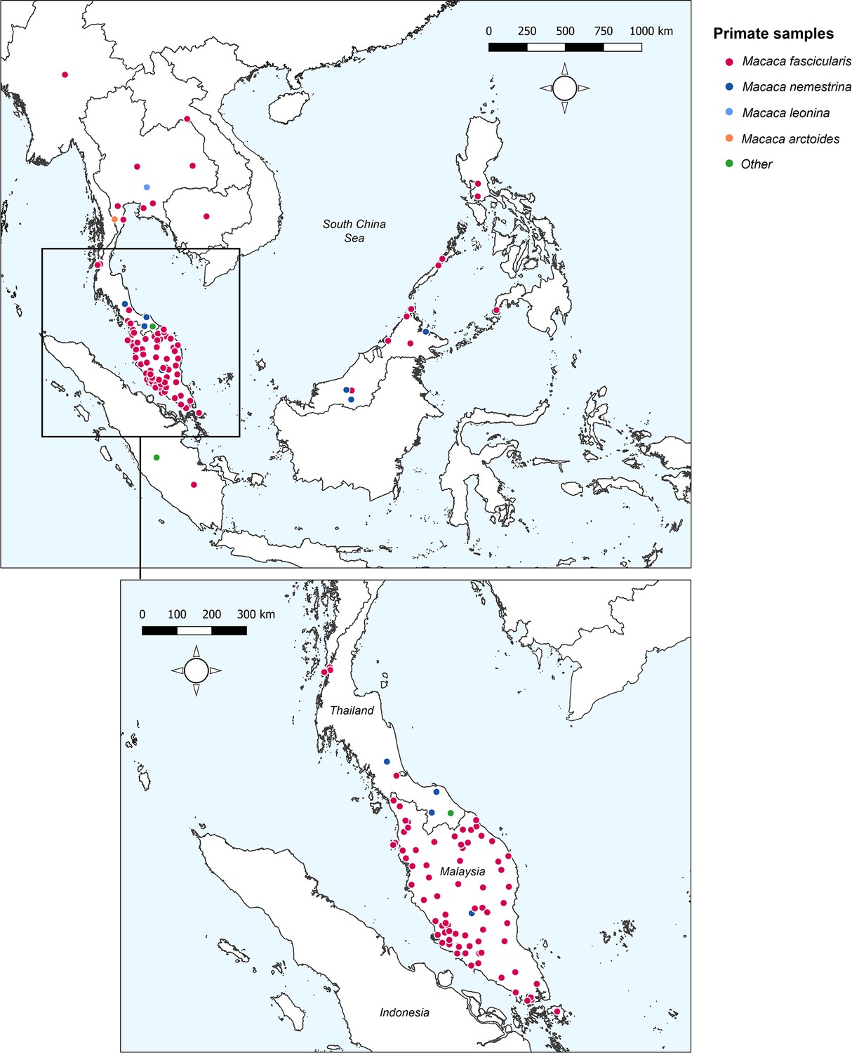
Sampling sites and primate species sampled across Southeast Asia.
‘Other’ includes Trachypithecus obscurus and undefined species from the genus Presbytis. Total surveys (n) = 148.
Figure 2
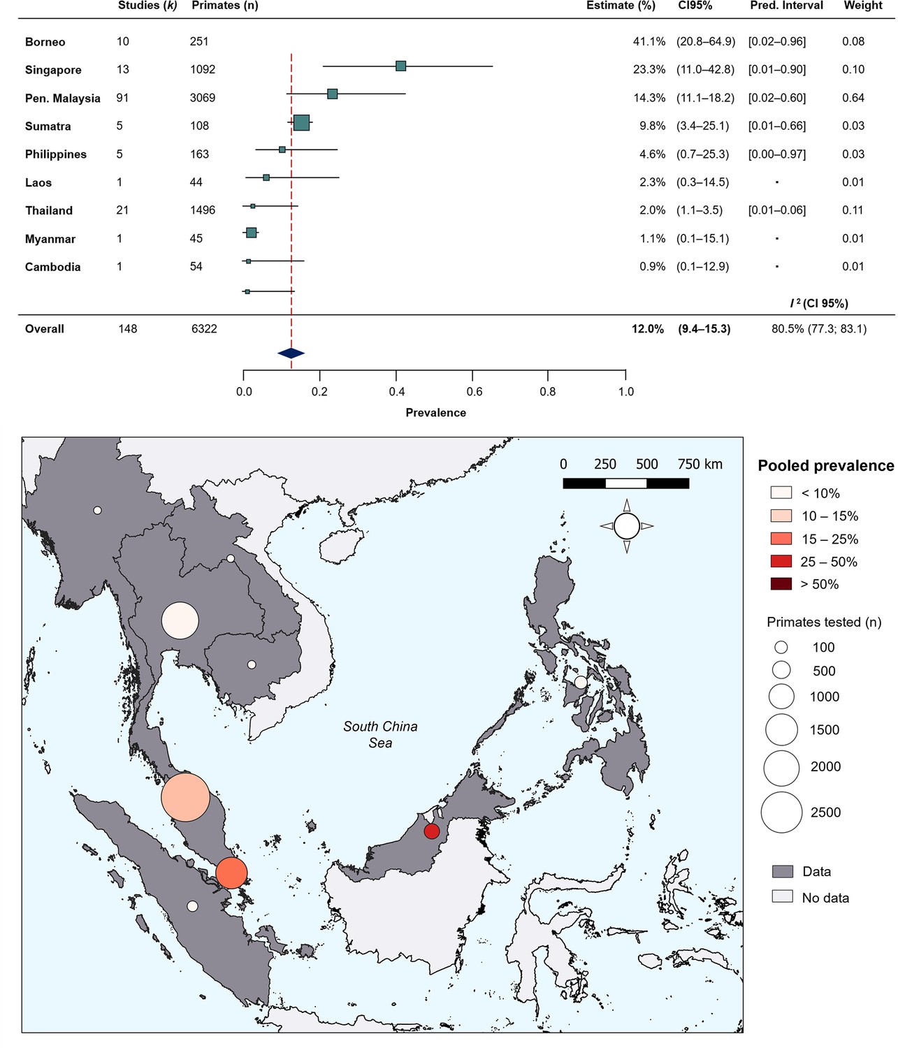
Random-effects meta-analysis of P. knowlesi prevalence across Southeast Asia.
(A) Forest plot of pooled estimates for P. knowlesi prevalence (%) in all non-human primates tested (n=6322) across Southeast Asia, disaggregated by species and sampling site (k=148). Random-effects meta-analysis sub-grouped by region, with 95% confidence intervals and prediction intervals. (B) Map of regional prevalence estimates for P. knowlesi prevalence in NHP in Southeast Asia from meta-analysis. Point colour denotes pooled estimate (%). Size denotes total primates tested per region (n). Shading indicates data availability.
Figure 3
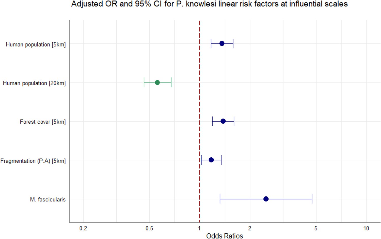
Multivariable regression results.
Spatial scale denoted in square bracket. Canopy cover = %. Adjusted odds ratios (OR, dots) and 95% confidence intervals (CI95%, whiskers) for factors associated with P. knowlesi in NHPs at significant spatial scales. N=1354, accounting for replicate pseudo-sampling.
Appendix 1—figure 1
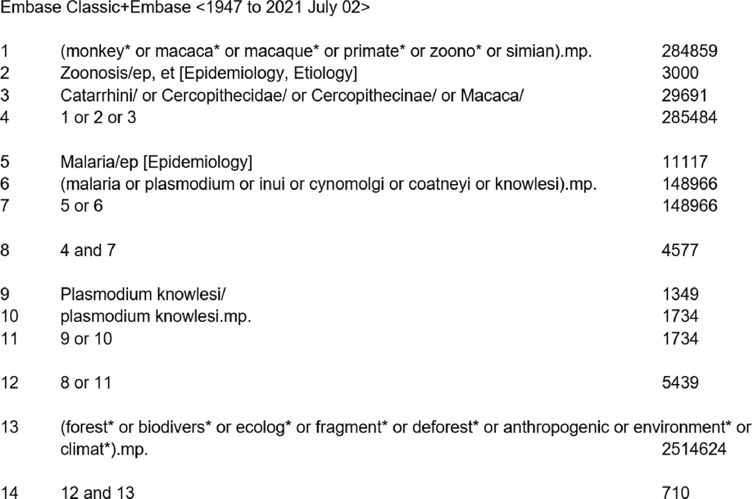
Search strategy for background research.
Appendix 1—figure 2
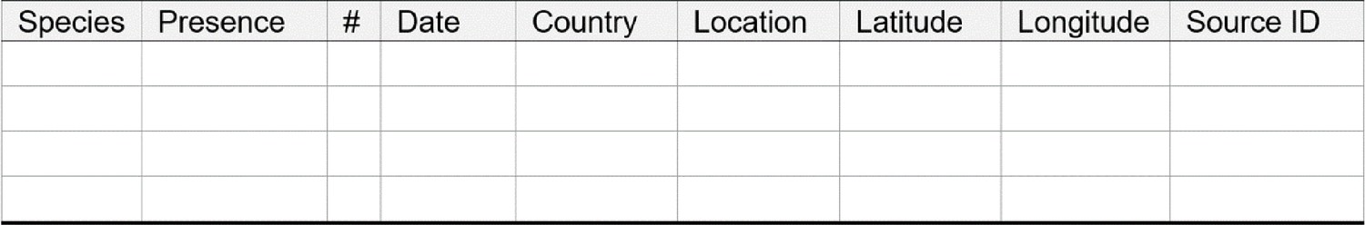
WHO Report primate data extraction form.
Appendix 1—figure 3
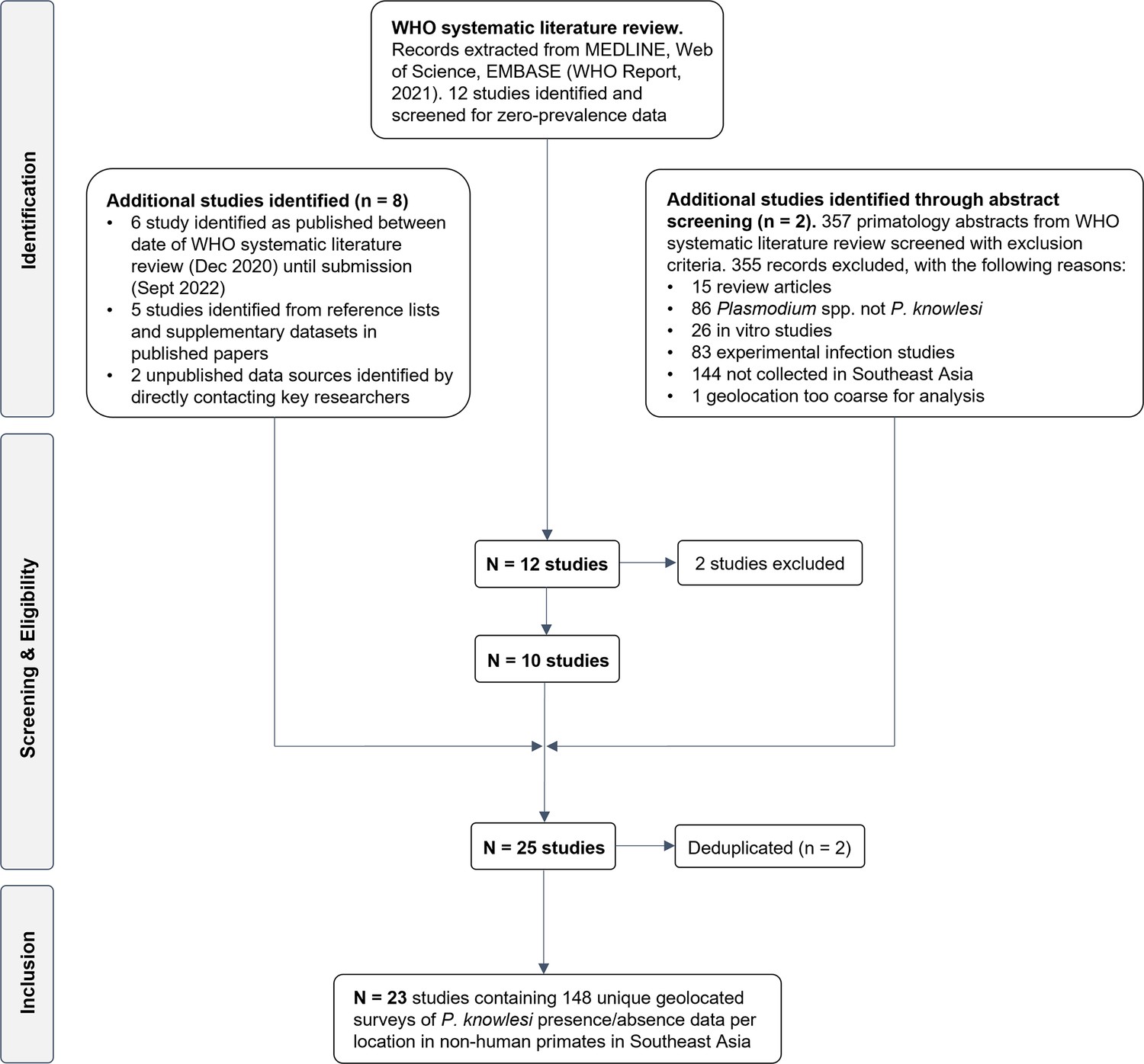
Flow chart illustrating study selection process.
Appendix 3—figure 1
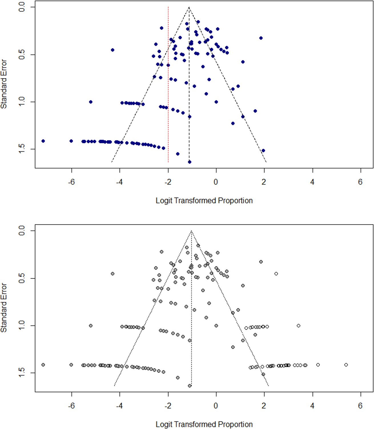
Assessment of small study effects in meta-analysis.
(A) Funnel plot of transformed prevalence (%) against standard error (SE) for study sites (B) Funnel plot with imputed data to illustrate asymmetry using trim-and-fill method.
Appendix 3—figure 2
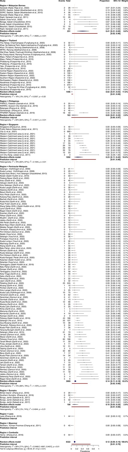
Forest plot of P. knowlesi prevalence (%) in all species of NHPs in Southeast Asia, disaggregated by species and sampling site, including 95% confidence intervals and individual study weighting.
Random-effects analysis, sub-grouped by region. N=148. Zarith et al. refers to personal correspondence derived from the reference Shahar, 2019.
Appendix 4—figure 1
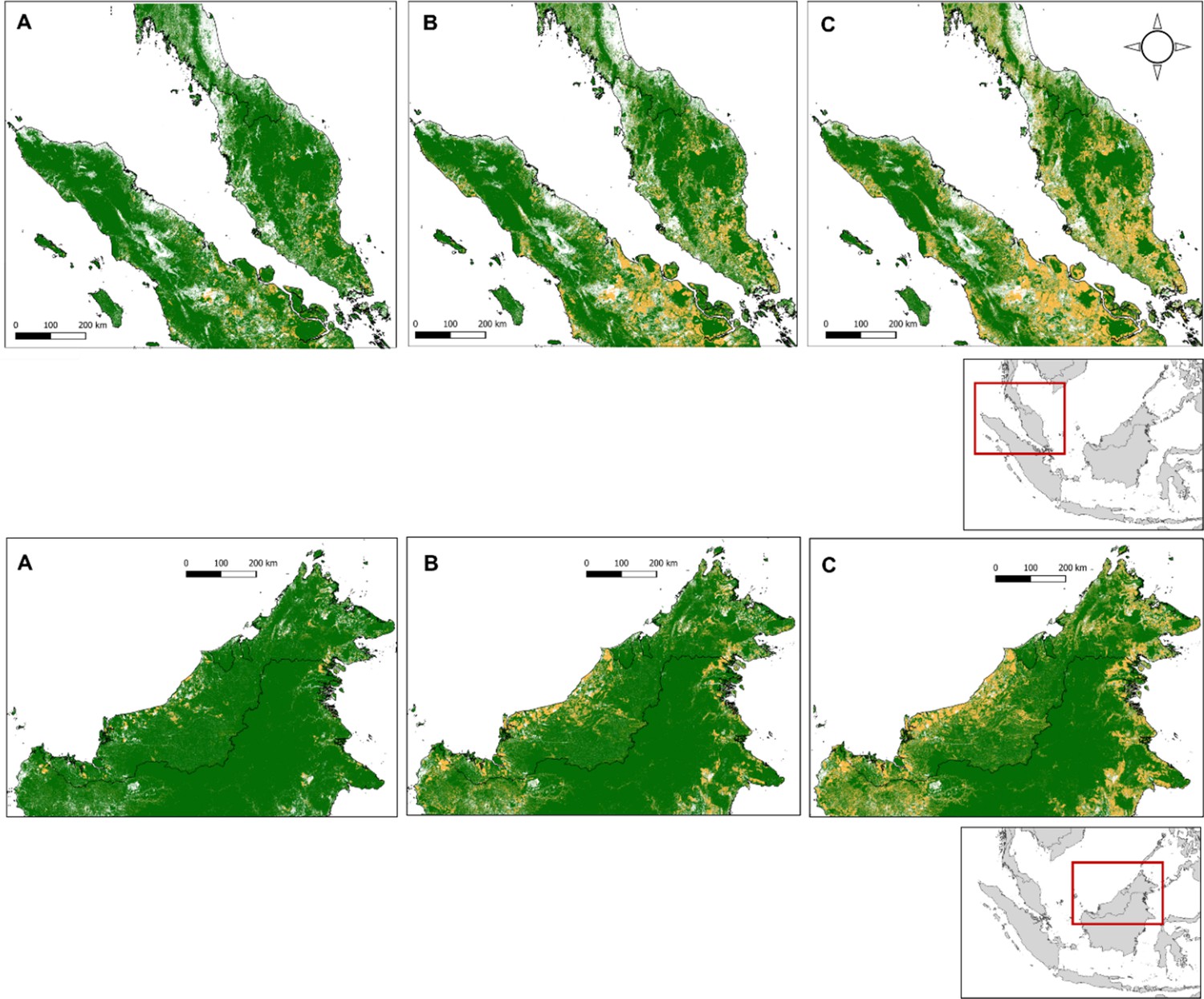
Recent forest loss in Peninsular Malaysia (first row) and Malaysian Borneo (secoond row), shown for the years (A) 2006 (B) 2012 and (C) 2019.
Appendix 4—figure 2
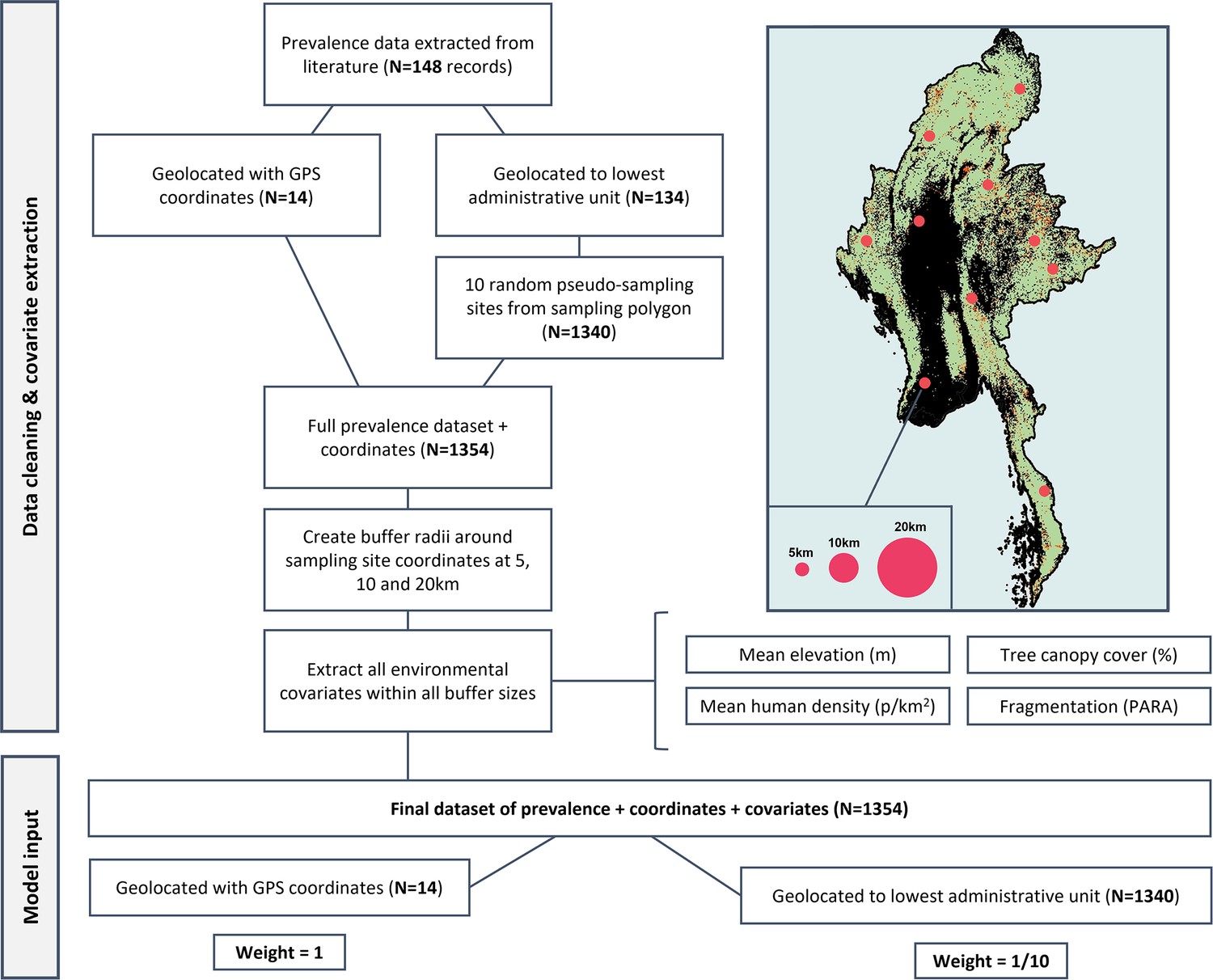
Flowchart of data processing.
Details of pseudo-sampling and environmental covariate extraction at multiple spatial scales to create final weighted dataset (N=1354).
Appendix 4—figure 3
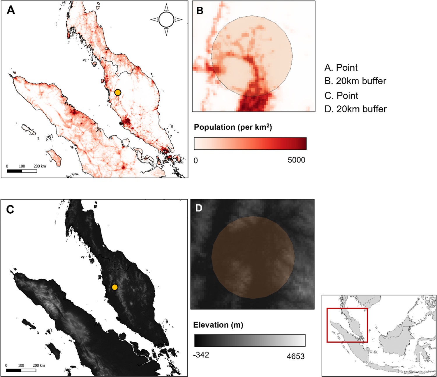
Example covariate resolutions in Peninsular Malaysia.
(A) Data point and (B) 20 km buffer over population density layer, 1 km resolution. (C) Data point and (D) 20 km buffer over SRTM elevation layer, 1 km resolution.
Appendix 4—figure 4
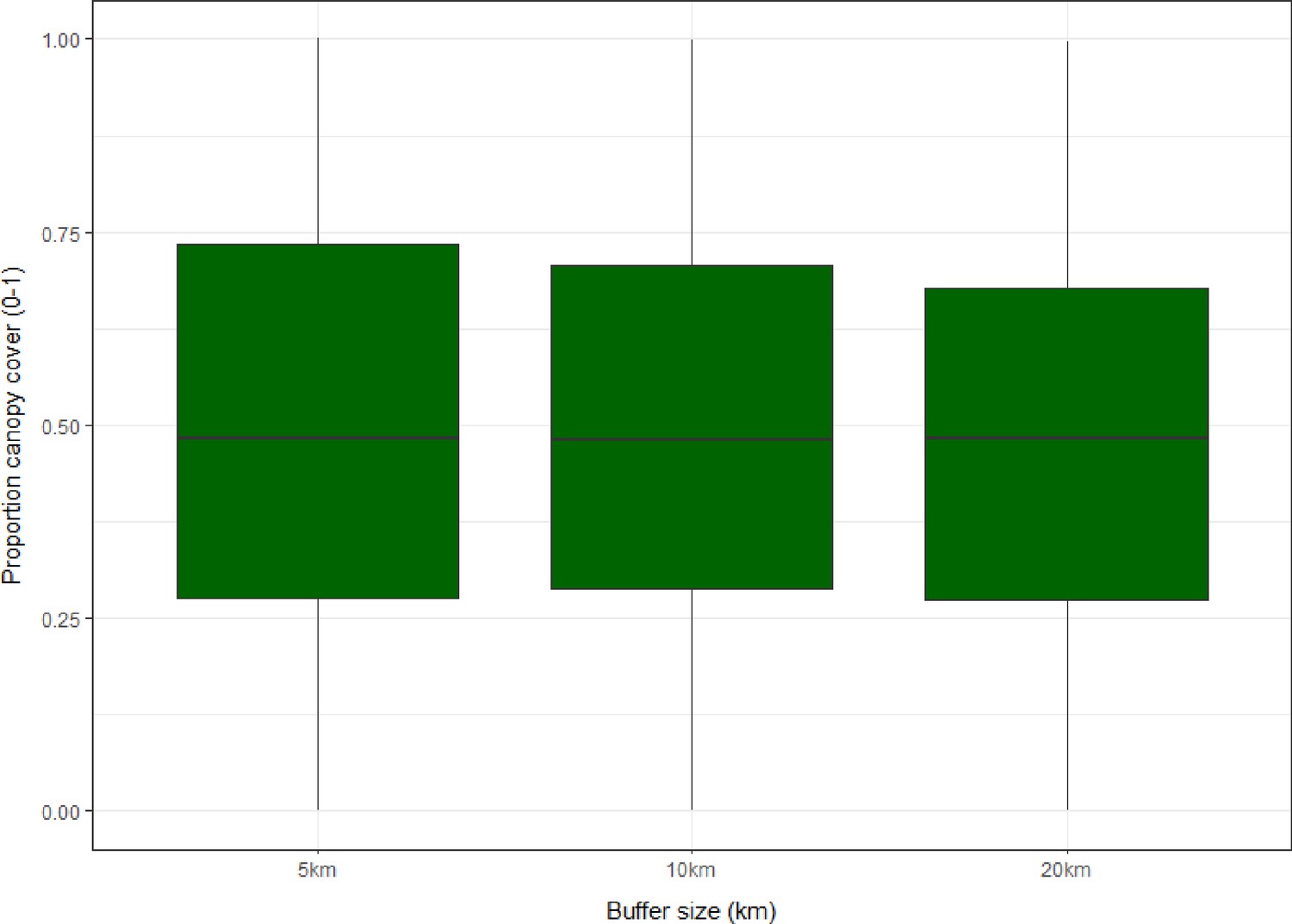
Boxplots showing distribution and interquartile range (IQR) of proportional forest cover (0–1) for sampling sites within 5, 10 and 20 km circular buffers across all sites (N=1354).
Appendix 4—figure 5
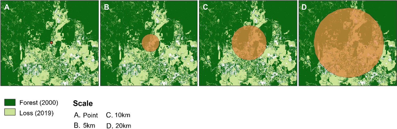
Examples of buffer zones around macaque sample sites.
Shown over forest cover for 2019 (Hansen et al., 2013).
Appendix 5—figure 1
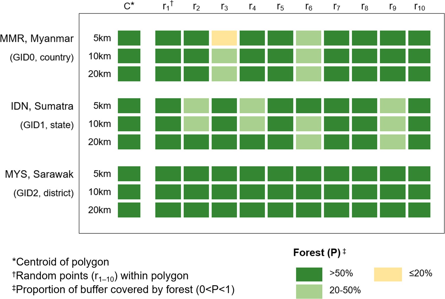
Sensitivity analysis comparing centroid forest cover to 10 randomly generated points, shown per radius for the largest polygon at each GADM level.
Appendix 5—figure 2
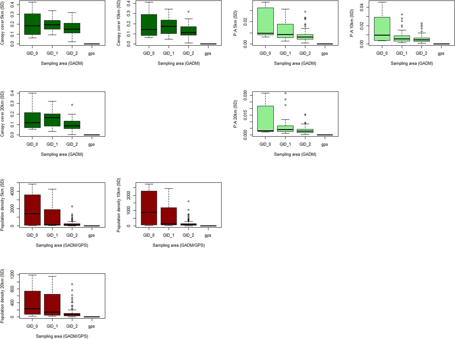
Boxplots of standard deviation in repeat sampling of covariates at multiple buffer and boundary sizes.
Standard deviation of environmental covariates across 10 sampling site realisations within 5/10/20km buffers, grouped by administrative boundary size or GPS coordinates. Shown for (A) canopy cover (%) (B) forest fragmentation (P: A ratio) and (C) human population density (p/km2).
Appendix 6—figure 1
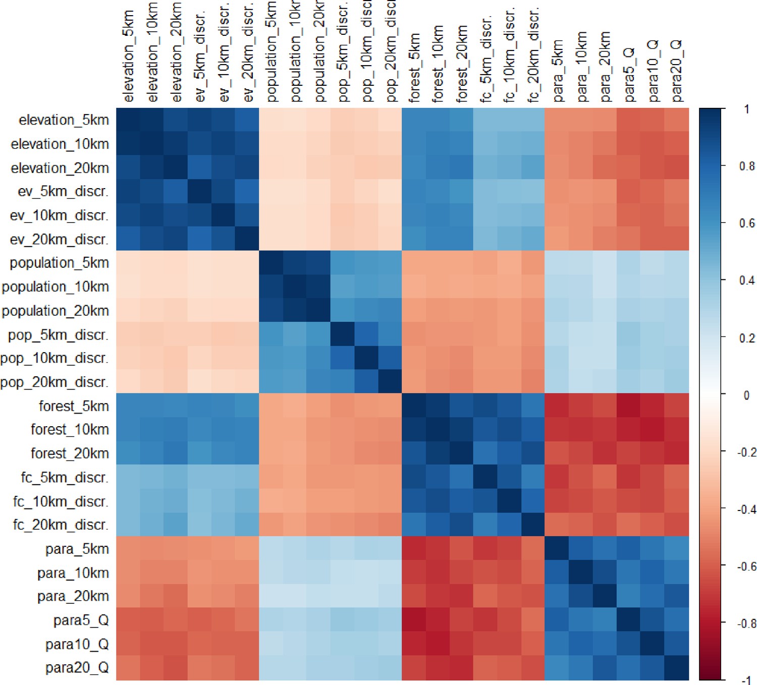
Spearman’s correlation matrix for all candidate covariates at all spatial scales (n=1354).
Appendix 6—figure 2
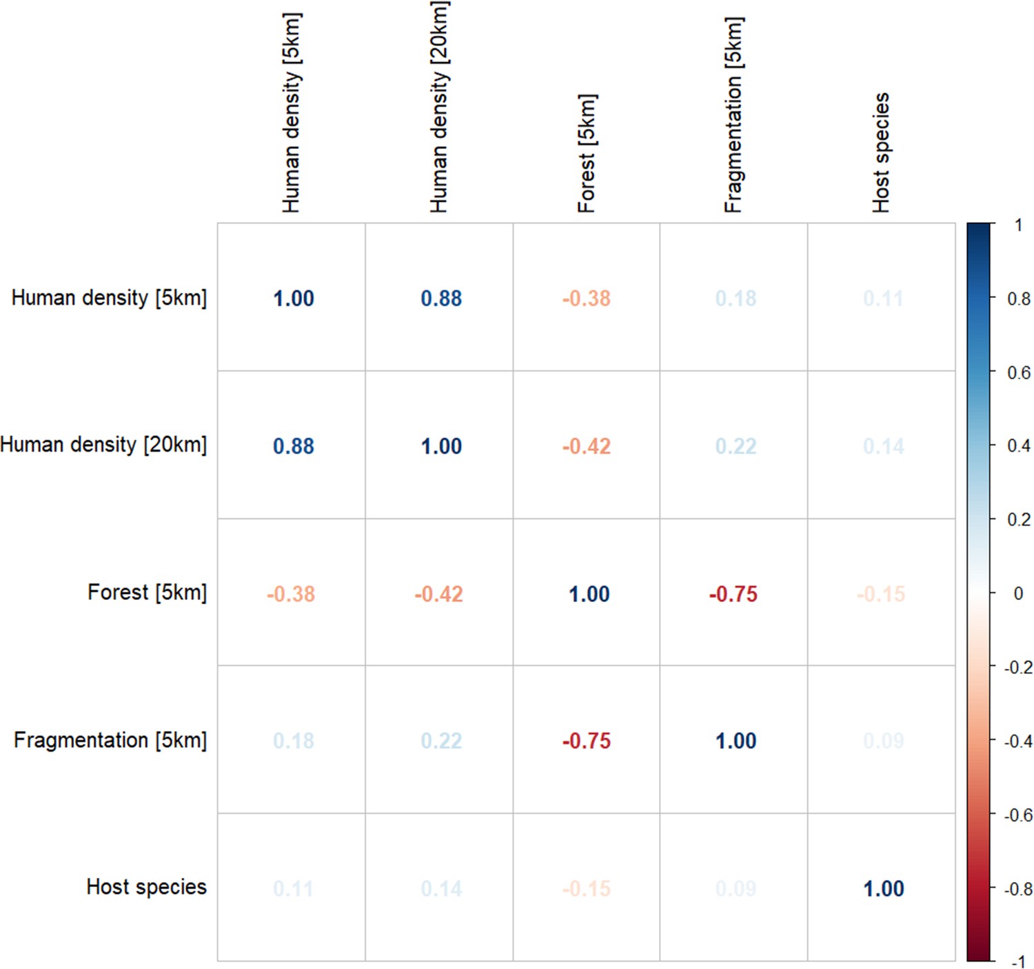
Spearman’s correlation matrix for covariates at selected spatial scales for final model inclusion (n=1354).
Percentage forest cover (5 km) and forest fragmentation (PARA, 5 km) show strong negative correlation (ρ=–0.75).
Appendix 6—figure 3
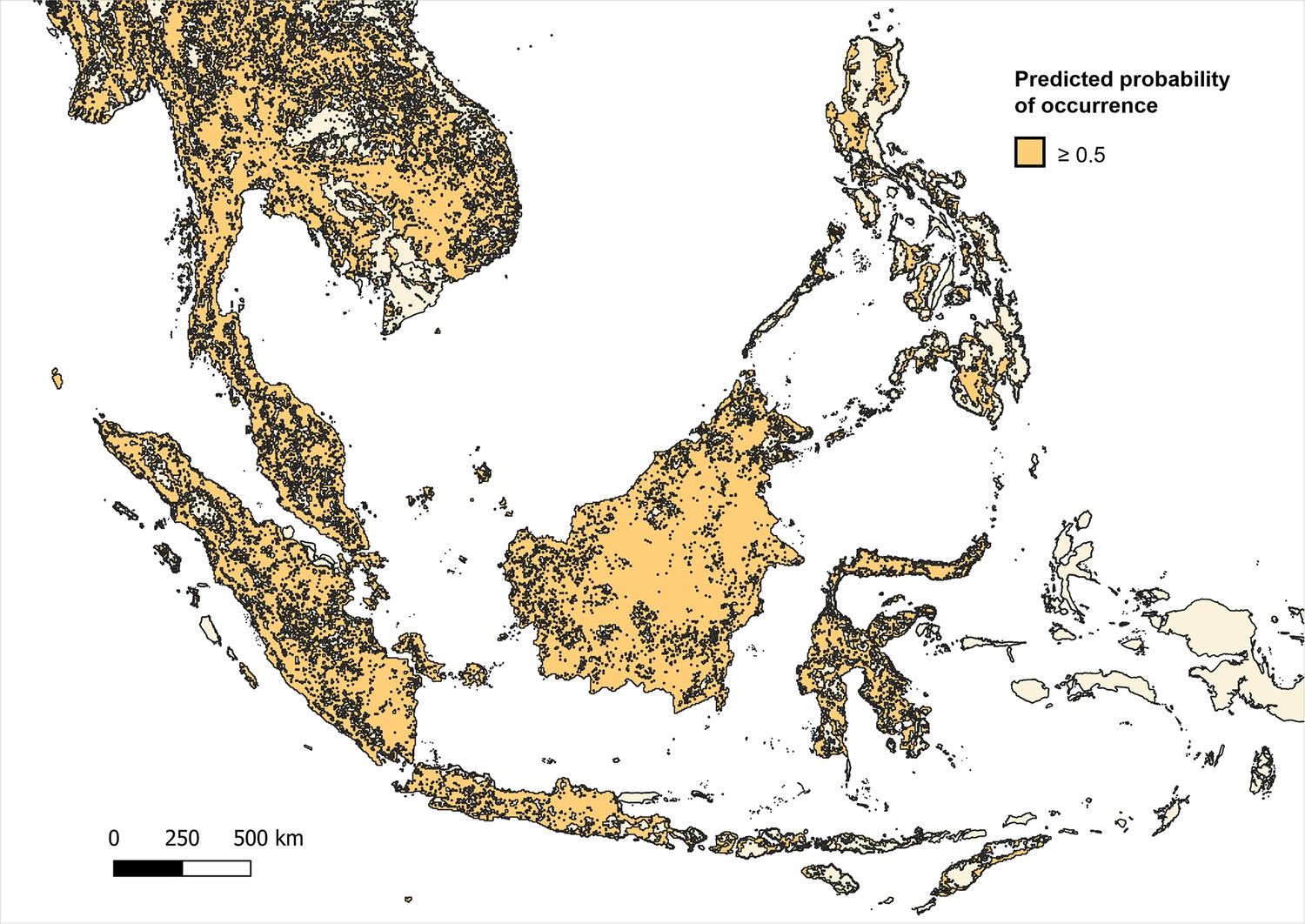
Distribution and habitat range of dominant macaque species (M. fascicularis, M. nemestrina, M. leonina) according to predicted probability of occurrence ≥0.5 (on a scale of 0–1.0) per 5x5 km pixel.
Appendix 6—figure 4
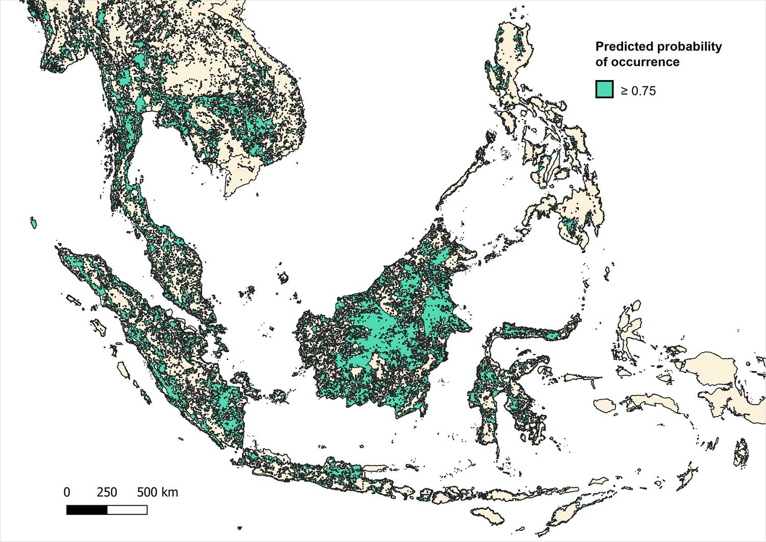
Distribution and habitat range of dominant macaque species (M. fascicularis, M. nemestrina, M. leonina) according to predicted probability of occurrence ≥0.75 (on a scale of 0–1.0) per 5x5 km pixel.
Appendix 6—figure 5
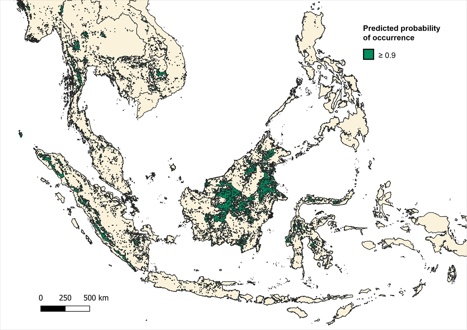
Predicted distribution and habitat range of all macaque species (M. fascicularis, M. nemestrina, M. leonina) according to predicted probability of occurrence ≥0.9 (on a scale of 0–1.0) per 5x5 km pixel.
Tables
Table 1
Spatial and temporal resolution (res.) and sources for environmental covariates.
Summary metrics extracted within 5, 10 and 20 km circular buffers.
| Covariate | Spatial res. | Temporal res. | Source |
|---|---|---|---|
| Human density (p/km2) | 1 km | 2012 | WorldPop, 2018 |
| Elevation (m) | 1 km | 2003 | SRTM 90 m Digital Elevation v4.1 Jarvis et al., 2008 |
| Tree cover (1/0)* | 30 m | Annual | Hansen’s Global Forest Watch Hansen et al., 2013 |
-
*
Derivatives: Proportion canopy cover (%), Perimeter: area ratio (PARA >0)
Appendix 1—table 1
Standardised definitions for qualitative primate characteristics.
| Variable | Category | Definition |
|---|---|---|
| Sampling | Routine | Animals collected for surveillance purposes or extracted from human–conflict zones; data collected opportunistically Shearer et al., 2016 |
| Study | Animals captured and sampled specifically for a study of Plasmodium spp and/or P. knowlesi | |
| Status | Captive | Animal resident in sanctuary or conservation park |
| Wild | Free-living animal, not registered/resident in any sanctuary | |
| Sanctuary | A wildlife sanctuary/rehabilitation centre housing key primate species Gamalo et al., 2019 | |
| Area | Forest | Areas that are uninhabited with extensive tree cover |
| Peri–domestic | As defined by the author. Example definitions as follows:
| |
| Agricultural | Animal located in agricultural areas, predominantly monoculture (e.g. orchard, plantation) Shahar, 2019 | |
| Urban | As defined by the author. Generally, areas with high human population density Li et al., 2021b |
Appendix 1—table 2
Characteristics of the included studies.
| Author | Year(s) | Country/region | N* | Sample† | Diagnostic | Target gene(s) | Primer |
|---|---|---|---|---|---|---|---|
| Lee et al., 2011 | 2004–2008 | Malaysia/Borneo | 108 | Study | Nested PCR | SSU-rRNA/csp/mtDNA | Kn1f/Kn3r |
| Seethamchai et al., 2008 | 2006 | Thailand | 99 | Study | Sequencing | A-type-SSU-rRNA/cytb | • |
| Vythilingam et al., 2008 | 2007 | Malaysia/Peninsular | 145 | Study | PCR/Sequencing | SSU-rRNA/csp | Pmk8/Pmkr9 |
| Zhang et al., 2016 | 2007 | Singapore | 40 | Study | PCR | • | • |
| 2007–2010 | Indonesia/Sumatra | 70 | Study | PCR | • | • | |
| 2011 | Cambodia | 54 | Study | PCR | • | • | |
| 2012 | Philippines | 68 | Study | PCR | • | • | |
| 2015 | Laos | 44 | Study | PCR/Sequencing | SSU-rRNA | PK18SF/PK18SRc | |
| Jeslyn et al., 2011 | 2008 | Singapore | 13 | Routine | PCR/Sequencing | SSU-rRNA /csp | Pmk8/Pmkr9 |
| Ho et al., 2010 | 2008 | Malaysia/Peninsular | 107 | Routine | Nested PCR | SSU-rRNA | Pmk8/Pmkr9 |
| Li et al., 2021b | 2008–2017 | Singapore | 1039 | Routine | Nested PCR | SSU-rRNA | Pmk8/Pmkr9 |
| Putaporntip et al., 2010 | 2009 | Thailand | 655 | Study | Sequencing | cytb | • |
| Chang et al., 2011 | 2010 | Myanmar | 45 | Study | PCR | SSU-rRNA | • |
| Muehlenbein et al., 2015 | 2010 | Malaysia/Borneo | 41 | Study | PCR | mtDNA/AMA-1/MSP-1 | • |
| Shahar, 2019 ‡ | 2010–2017 | Malaysia/Peninsular | 1587 | Routine | Nested PCR | SSU-rRNA | • |
| § | 2013 | Malaysia/Peninsular | 15 | Study | PCR | • | • |
| § | 2013–2016 | Malaysia/Borneo | 25 | Study | Nested PCR | cytb | PKCBF/PKCBR |
| Saleh Huddin et al., 2019 | 2014 | Malaysia/Peninsular | 415 | Study | PCR/Sequencing | SSU-rRNA | Pmk8/Pmkr9 |
| Akter et al., 2015 | 2015 | Malaysia/Peninsular | 70 | Routine | PCR/Sequencing | A-type-SSU-rRNA | Pmk8/Pmkr9 |
| Amir et al., 2020 | 2016 | Malaysia/Peninsular | 103 | Routine | Nested PCR | SSU-rRNA | PkF1140/PkR1550 |
| Gamalo et al., 2019 | 2017 | Philippines | 95 | Study | Nested PCR | SSU-rRNA | Kn1f/Kn3r |
| Fungfuang et al., 2020 | 2017–2019 | Thailand | 93 | Study | Nested PCR | SSU-rRNA | Kn1f/Kn3r |
| Nada-Raja et al., 2022 | 2018 | Malaysia/Borneo | 73 | Study | Nested PCR | SSU-rRNA/csp/mtDNA | Kn1f/Kn3r |
| Yusuf et al., 2022 | 2016–2019 | Malaysia | 419 | Study | Nested PCR | SSU-rRNA | Kn1f/Kn3r |
| Zamzuri et al., 2020 | 2018 | Malaysia/Peninsular | 212 | Routine | PCR | • | • |
| Kaewchot et al., 2022 | 2019 | Thailand | 649 | Study | Nested PCR | SSU-rRNA | Pmk8/Pmkr9 |
| Salwati et al., 2017 | 2015 | Indonesia/Sumatra | 38 | Study | PCR/Sequencing | • | • |
-
*
N=number of primates sampled.
-
†
Animal trapped either on routine or study basis.
-
‡
Unpublished, personal correspondence (p/c).
-
§
Danau Girang Field Centre, p/c from Dr Salgado Lynn.
Appendix 1—table 3
Published studies of P. knowlesi infections (n) in non-human primate species collected (N) in Southeast Asia, grouped by region and author.
-
*
Macaca-leonina (Northern Pig-tailed macaque, recently classified as separate species).
-
†
Presbytis spp.
-
‡
Trachypithecus obscurus (Dusky leaf monkey).
Appendix 1—table 4
Characteristics of primates tested and number/percentage of confirmed P. knowlesi infections (Pk+).
| N | (%)* | Pk+ | Pk+ (%)† | CI95% ‡ | ||
|---|---|---|---|---|---|---|
| Species | M. fascicularis | 5720 | (90.5%) | 745 | 13.0% | (12.2–13.9) |
| M. nemestrina | 532 | (8.4%) | 26 | 4.9% | (3.4–7.1) | |
| M. leonina | 25 | (0.4%) | 0 | 0.0% | (0.0–13.3) | |
| M. arctoides | 36 | (0.6%) | 1 | 2.8% | (0.5–14.2) | |
| T. obscurus | 7 | (0.1%) | 1 | 14.3% | (2.6–51.3) | |
| Presbytis spp. | 2 | (0.03%) | 0 | 0.0% | (0.0–65.8) | |
| Area | Forest | 1740 | (27.5%) | 253 | 14.5% | (13.0–16.3) |
| Agriculture | 491 | (7.8%) | 72 | 14.7% | (11.8–18.1) | |
| Peri-domestic | 2192 | (34.7%) | 341 | 15.6% | (14.1–17.1) | |
| Urban | 1143 | (18.1%) | 56 | 4.9% | (3.8–6.3) | |
| Sanctuary | 109 | (1.7%) | 5 | 4.6% | (2.0–10.3) | |
| Unspecified | 647 | (10.2%) | 46 | 7.1% | (5.4–9.4) | |
| Status | Wild | 6183 | (97.8%) | 768 | 12.4% | (11.6–13.3) |
| Captive | 139 | (2.2 %) | 5 | 3.6% | (1.5–8.1) | |
| Region | Pen. Malaysia | 3069 | (48.5%) | 473 | 15.4% | (14.2–16.7) |
| Borneo | 251 | (4.0%) | 119 | 47.4% | (41.3–53.6) | |
| Sumatra | 108 | (1.7%) | 6 | 5.5% | (2.6–11.6) | |
| Thailand | 1496 | (23.7%) | 8 | 0.5% | (0.3–1.1) | |
| Philippines | 163 | (2.6 %) | 18 | 11.0% | (7.1–16.8) | |
| Singapore | 1092 | (17.3%) | 148 | 13.6% | (11.7–15.7) | |
| Cambodia | 54 | (0.9%) | 0 | 0.0% | (0.0–6.6) | |
| Laos | 44 | (0.7%) | 1 | 2.3% | (0.4–11.8) | |
| Myanmar | 45 | (0.7%) | 0 | 0.0% | (0.0–7.9) | |
| Total | 6322 | (100%) | 773 | 12.2% | (11.4–13.1) |
-
*
Percentage of total number of primates tested (column %).
-
†
Proportion of N positive for P. knowlesi (row %).
-
‡
95% confidence interval (CI95%) calculated in R using count and sample size (binomial distribution).
Appendix 2—table 1
JBI criteria for assessing bias in meta-analyses of prevalence studies.
| Criteria | Yes | No | Unclear | N/A | |
|---|---|---|---|---|---|
| Q1 | Was the sample frame appropriate to address the target population? | ||||
| Q2 | Were study participants sampled in an appropriate way? | ||||
| Q3 | Was the sample size adequate? | ||||
| Q4 | Were the study subjects and the setting described in detail? | ||||
| Q5 | Was the data analysis conducted with sufficient coverage of the identified sample? | ||||
| Q6 | Were valid methods used for the identification of the condition? | ||||
| Q7 | Was the condition measured in a standard, reliable way for all participants? | ||||
| Q8 | Was there appropriate statistical analysis? | ||||
| Q9 | Was the response rate adequate, and if not, was the low response rate managed appropriately? | ||||
Appendix 2—table 2
Example rationale for quality appraisal.
| Sample question | Example | Assessment | |
|---|---|---|---|
| Q1 | Was the sample frame appropriate to address the target | Wild animal | Yes |
| population? | Captive animal | No | |
| Not specified | Uncertain | ||
| Q2 | Were study participants sampled in an appropriate way? | Trapped for study | Yes |
| Routine collection | No | ||
| Not specified | Uncertain | ||
| Q9 | Was the response rate adequate? | Primate data | N/A |
Appendix 3—table 1
Sensitivity analysis for transformation of P. knowlesi prevalence estimate under random-effects model, shown overall and for Thailand subgroup analysis.
| Method | Overall (k=148) | Subgroup (Thailand, k=21) | ||
|---|---|---|---|---|
| P* | CI95% | P | CI95% | |
| Freeman-Turkey double arcsine | 0.0943 | (0.0641–0.1284) | 0.0000 | (0.0000–0.0000) |
| Logit | 0.1199 | (0.0935–0.1526) | 0.0199 | (0.0113–0.0346) |
| Untransformed | 0.1415 | (0.1101–0.1730) | 0.0022 | (0.0000–0.0059) |
-
*
Estimated proportion
Appendix 4—table 1
Environmental covariates assembled for regression analysis.
Summary values extracted for each covariate within 5, 10, and 20 km circular buffers during processing.
| Covariate | Description | Metric | Resolution | Processing | Source | |
|---|---|---|---|---|---|---|
| Spatial | Temporal | |||||
| Population | UN-adjusted gridded posterior population model estimates at 30 arc-seconds resolution | Person count/1 km2 | 1 km | 2000 2012 2019 | Population density reclassified as high/low (≤300 persons/km2) in QGIS | WorldPop, 2018 Downloaded as tiff files per country in AOI for years 2000/2012/2019 |
| Elevation | Mean height above sea level | m | 1 km | 2003 | Mean and SD of continuous elevation per radii. Mean-centred and scaled. Categorised into discrete classifications: low (≤200 m), moderate (200–500 m) or high elevation (>500 m) | NASA SRTM 90 m Digital Elevation Database v4.1 (CGIAR-CSI) Jarvis et al., 2008. Downloaded as a tiff file at 1 km resampled resolution |
| Forest | Percentage canopy cover per grid cell. Derived from tree cover (vegetation >5 m) and loss (forested to non-forested) | 0–1 | 30 m | Annual 2006–2020 | Tree cover classified as ≥50% crown density per raster cell, generating binary raster (1=forest, 0=non-forest). Annual cover calculated by subtracting cumulative loss per year 2006–2019. Data records matched to reclassified tile by geolocation and year. Posterior proportions categorised as high (>50%) medium (20–50%) or low (≤20%) | Hansen’s Global Forest Watch, 30 m resolution Landsat imagery Hansen et al., 2013. Tiles downloaded as tiff files for each year 2006–2019 to cover AOI |
| Fragmentation (perimeter: area ratio, PARA) | Perimeter length (m) to patch area (m2) ratio for contiguous forest cover McGarigal et al., 2021 within buffer | PARA >0 | 30 m | Annual 2006–2020 | Extracted from annual reclassified tree cover rasters within 5, 10 and 20 km circular buffers Output categorised into quartiles | Hansen’s Global Forest Watch Hansen et al., 2013 (as above) |
Appendix 4—table 2
Summary of forest cover data (N=1480).
| Mean | SD | Range | |
|---|---|---|---|
| Forest cover (5 km) | 50.20% | ±29.29% | 0.00–100.00% |
| Forest cover (10 km) | 49.68% | ±27.30% | 0.00–99.96% |
| Forest cover (20 km) | 48.29% | ±25.35% | 0.00–99.64% |
| Total | 1480 (100%) |
Appendix 5—table 1
Geo-positioning of available primate survey data.
| Resolution/GADM* | Records/n | Primates/N | Min. (km2)† | Max. (km2) | |
|---|---|---|---|---|---|
| Polygon | Country/GID0 | 6 (4.9%) | 853 (17.3%) | 700 | 77,650 |
| State/GID1 | 40 (22.0%) | 2699 (32.2%) | 130 | 87,860 | |
| District/GID2 | 88 (61.8%) | 2433 (43.6%) | 270 | 15,890 | |
| Point | GCS ‡ | 14 (11.4%) | 337 (6.8%) | – | – |
| Total | 148 (100%) | 4931 (100%) |
-
*
Administrative boundaries, as classified by GADM (v3.6).
-
†
Minimum and maximum size (km2) of polygons containing P. knowlesi data at each admin level.
-
‡
Geographic Coordinate System.
Appendix 6—table 1
Bivariable analysis for P. knowlesi in NHP against all covariates at all spatial scales (N=1354).
| Bivariable analysis | ||||
|---|---|---|---|---|
| Variable | Crude OR | CI95% | p value† | |
| Elevation (m) * | ||||
| ≤5 km | 1.18 | (1.07–1.28) | 0.000562 | |
| ≤10 km | 1.20 | (1.09–1.31) | 0.0001246 | |
| ≤20 km | 1.22 | (1.11–1.33) | 7.23E-05 | |
| Human density (p/km2) * | ||||
| ≤5 km | 0.84 | (0.77–0.92) | 4.72E-05 | |
| ≤10 km | 0.75 | (0.68–0.82) | 2.70E-12 | |
| ≤20 km | 0.71 | (0.63–0.79) | 1.37E-12 | |
| Forest cover (%) * | ||||
| ≤5 km | 1.34 | (1.21–1.49) | 1.86E-08 | |
| ≤10 km | 1.41 | (1.26–1.57) | 6.51E-10 | |
| ≤20 km | 1.47 | (1.30–1.67) | 8.66E-10 | |
| Fragmentation (PARA) * | ||||
| ≤5 km | 0.85 | (0.76–0.95) | 0.003944 | |
| ≤10 km | 0.69 | (0.60–0.80) | 1.80E-07 | |
| ≤20 km | 0.67 | (0.57–0.79) | 5.14E-07 | |
| PARA2 * | Quadratic term | |||
| ≤5 km | 0.69 | (0.60–0.80) | 0.10 | 2.06E-06 |
| ≤10 km | 0.64 | (0.55–0.74) | 0.08 | 2.65E-08 |
| ≤20 km | 0.67 | (0.57–0.78) | 0.03 | 2.78E-06 |
| Host species | ||||
| Other | Ref | |||
| M. fascicularis | 2.37 | (1.25–4.60) | 0.007971 | |
-
*
Continuous variable, mean-centred and scaled.
-
†
p value derived from Likelihood ratio test (LRT).
Appendix 6—table 2
Multivariable binomial regression analysis of P. knowlesi prevalence in NHP with environmental covariates at influential spatial scales, full dataset (N=1354).
AIC = 1229.8.
| Multivariable analysis | ||||
|---|---|---|---|---|
| Variable | Radius | aOR * | CI95% | p value † |
| Human density (p/km2) ‡ | ||||
| ≤5km | 1.36 | (1.16–1.58) | 1.082E-04 | |
| ≤20 km | 0.56 | (0.46–0.67) | 1.311E-10 | |
| Forest cover (%) ‡ | ||||
| ≤5 km | 1.38 | (1.19–1.60) | 2.046E-05 | |
| Fragmentation (PARA) ‡ | ||||
| ≤5 km | 1.17 | (1.02–1.34) | 0.0281 | |
| Host species | ||||
| Other | Ref | |||
| M. fascicularis | 2.50 | (1.31–4.85) | 0.005121 | |
-
*
Odds Ratios adjusted for all other variables in the table (aOR). Radius calculated as distance from sample point.
-
†
p value derived from Likelihood ratio test (LRT).
-
‡
Continuous variable, mean-centred and scaled. OR shown per 1 SD increase.
Appendix 6—table 3
Admin boundary sensitivity analysis.
Binomial regression analysis of P. knowlesi prevalence in NHP for datapoints assigned to GPS or small sized administrative boundaries (excluding country data) (N=1324).
| AIC = 1221.9 | Multivariable analysis | ||
|---|---|---|---|
| aOR | CI 95% | p value (Wald test)* | |
| Human density [5 km] | 1.36 | (1.16–1.58) | *** |
| Human density [20 km] | 0.56 | (0.46–0.67) | *** |
| Forest cover (%) [5 km] | 1.38 | (1.19–1.60) | *** |
| Fragmentation (PARA) [5 km] | 1.18 | (1.02–1.34) | * |
| Host group Other M. fascicularis | REF 2.51 | (1.–.31–4.85) | ** |
-
*
Signif. codes: 0 ‘***’ 0.001 ‘**’ 0.01 ‘*’ 0.05 ‘.’ 0.1 ‘ ’ 1.
Appendix 6—table 4
Distribution of standard deviations across 10 environmental covariates per prevalence data point for landscape variables at all spatial scales (N=1354).
| Covariate | Mean | Range | Median | IQR |
|---|---|---|---|---|
| Canopy [5 km]* | 0.1588 | 0.0000–0.4237 | 0.1534 | 0.1039–0.2277 |
| Canopy [10 km] | 0.1319 | 0.0000–0.4124 | 0.1177 | 0.0827–0.1891 |
| Canopy [20 km] | 0.1051 | 0.0000–0.3999 | 0.0921 | 0.0541–0.1635 |
| Fragmentation [5 km]* | 0.0083 | 0.0000–0.0375 | 0.0063 | 0.0041–0.0094 |
| Fragmentation [10 km] | 0.0061 | 0.0000–0.0455 | 0.0043 | 0.0025–0.0071 |
| Fragmentation [20 km] | 0.0041 | 0.0000–0.0316 | 0.0027 | 0.0017–0.0047 |
-
*
Spatial scales selected in final variables.
Appendix 6—table 5
Tree canopy cover sensitivity analysis.
Binomial regression of P. knowlesi prevalence in NHP for datapoints, with data where SD < ½ the maximum for tree canopy within 5 km (N=814).
| AIC = 771.1 | Multivariable analysis | ||
|---|---|---|---|
| aOR | CI 95% | p value (Wald test)* | |
| Human density [5 km] | 0.90 | (0.67–1.20) | - |
| Human density [20 km] | 0.72 | (0.50–1.01) | . |
| Forest cover (%) [5 km] | 1.70 | (1.30–2.24) | *** |
| Fragmentation (PARA) [5 km] | 1.38 | (1.01–1.88) | * |
| Host group Other M. fascicularis | REF 2.63 | (1.35–5.21) | ** |
-
*
Signif. codes: 0 ‘***’ 0.001 ‘**’ 0.01 ‘*’ 0.05 ‘.’ 0.1 ‘-’ 1.
Appendix 6—table 6
Landscape fragmentation sensitivity analysis.
Binomial regression of P. knowlesi prevalence in NHP for datapoints, with datapoints where SD < ½ the maximum for fragmentation within 5 km (N=1134).
| AIC = 982.9 | Multivariable analysis | ||
|---|---|---|---|
| aOR | CI 95% | p value (Wald test)* | |
| Human density [5 km] | 0.91 | (0.69–1.18) | - |
| Human density [20 km] | 0.69 | (0.52–0.93) | * |
| Forest cover (%) [5 km] | 1.31 | (1.08–1.60) | ** |
| Fragmentation (PARA) [5 km] | 1.18 | (0.90–1.54) | - |
| Host group Other M. fascicularis | REF 2.52 | (1.33–4.87) | ** |
-
*
Signif. codes: 0 ‘***’ 0.001 ‘**’ 0.01 ‘*’ 0.05 ‘.’ 0.1 ‘ ’ 1.
Appendix 6—table 7
Macaque habitat suitability sensitivity analysis.
Binomial regression of P. knowlesi prevalence in NHP for datapoints, including only datapoints with 5 km buffers that intersect with areas with ≥0.5 probability of predicted macaque occurrence (N=1331).
| AIC = 1197.2 | Multivariable analysis | ||
|---|---|---|---|
| aOR | CI 95% | p value (Wald test)* | |
| Human density [5 km] | 1.32 | (1.13–1.54) | *** |
| Human density [20 km] | 0.55 | (0.45–0.66) | *** |
| Forest cover (%) [5 km] | 1.30 | (1.12–1.52) | *** |
| Fragmentation (PARA) [5 km] | 1.12 | (0.97–1.29) | - |
| Host group Other M. fascicularis | REF 2.48 | (1.31–4.82) | ** |
-
*
Signif. codes: 0 ‘***’ 0.001 ‘**’ 0.01 ‘*’ 0.05 ‘.’ 0.1 ‘ ’ 1.
Appendix 6—table 8
Macaque habitat suitability sensitivity analysis.
Binomial regression of P. knowlesi prevalence in NHP for datapoints, including only datapoints with 5 km buffers that intersect with areas with ≥0.75 probability of predicted macaque occurrence (N=1177).
| AIC = 1115.5 | Multivariable analysis | ||
|---|---|---|---|
| aOR | CI 95% | p value (Wald test)* | |
| Human density [5 km] | 1.34 | (1.14–1.58) | *** |
| Human density [20 km] | 0.57 | (0.47–0.69) | *** |
| Forest cover (%) [5 km] | 1.23 | (1.04–1.47) | * |
| Fragmentation (PARA) [5 km] | 1.04 | (0.86–1.24) | - |
| Host group Other M. fascicularis | REF 2.69 | (1.38–5.38) | ** |
-
*
Signif. codes: 0 ‘***’ 0.001 ‘**’ 0.01 ‘*’ 0.05 ‘.’ 0.1 ‘ ’ 1.
Appendix 6—table 9
Macaque habitat suitability sensitivity analysis.
Binomial regression of P. knowlesi prevalence in NHP for datapoints, including only datapoints with 5 km buffers that intersect with areas with ≥0.9 probability of predicted macaque occurrence (N=567).
| AIC = 685.2 | Multivariable analysis | ||
|---|---|---|---|
| aOR | CI 95% | p value (Wald test)* | |
| Human density [5 km] | 1.86 | (1.49–2.32) | *** |
| Human density [20 km] | 0.36 | (0.26–0.49) | *** |
| Forest cover (%) [5 km] | 1.47 | (1.14–1.90) | ** |
| Fragmentation (PARA) [5 km] | 1.35 | (1.02–1.77) | * |
| Host group Other M. fascicularis | REF 3.13 | (1.50–6.75) | ** |
-
*
Signif. codes: 0 ‘***’ 0.001 ‘**’ 0.01 ‘*’ 0.05 ‘.’ 0.1 ‘ ’ 1.
Additional files
Download links
A two-part list of links to download the article, or parts of the article, in various formats.
Downloads (link to download the article as PDF)
Open citations (links to open the citations from this article in various online reference manager services)
Cite this article (links to download the citations from this article in formats compatible with various reference manager tools)
Landscape drives zoonotic malaria prevalence in non-human primates
eLife 12:RP88616.
https://doi.org/10.7554/eLife.88616.4


