Stochastic characterization of navigation strategies in an automated variant of the Barnes maze
- Center for Functional Connectomics, Brain Science Institute, Korea Institute of Science and Technology (KIST), Republic of Korea
- Division of Bio-Medical Science and Technology, KIST School, Korea University of Science and Technology (UST), Republic of Korea
Figures
Figure 1 with 1 supplement
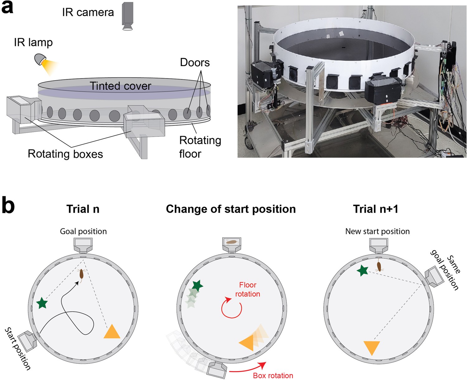
Design and operation of the automated variant of the Barnes maze.
(a) Scheme (left) and picture (right) showing a side view of the apparatus with its different components. The environmental cues are restricted to objects within the arena as the tinted cover blocks visual cues from the surrounding room. (b) Scheme showing the operation of the apparatus. A new start position is set by rotating the arena. The goal box is simultaneously moved to align with the goal location. The spatial information remains consistent across trials since the guiding objects are rotated together with the arena.
Figure 1—figure supplement 1
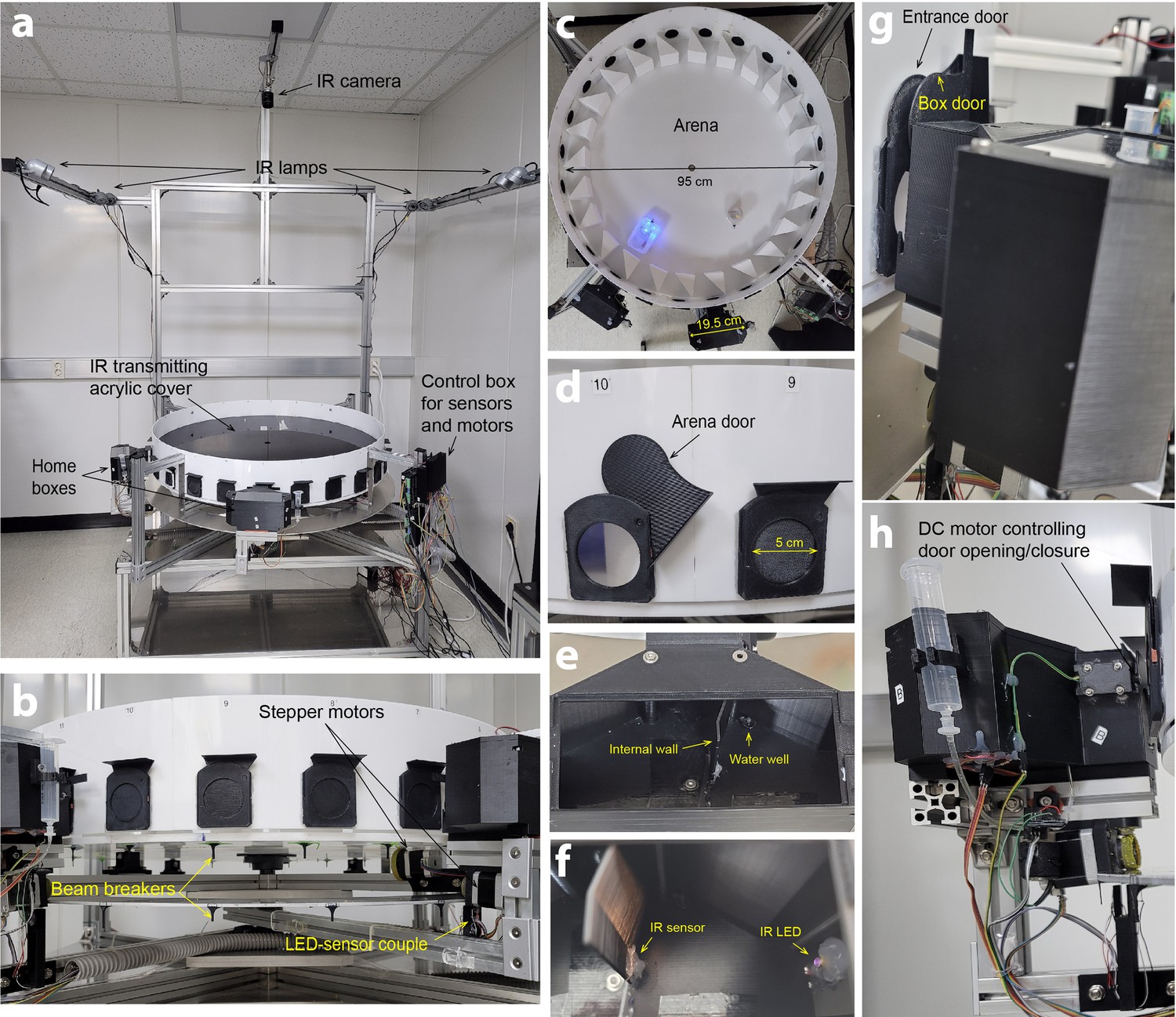
Detailed view of the automated variant of the Barnes maze.
(a–c) Pics of the entire apparatus (a) and of the side (b) and top views (c) of the apparatus. (d) Zoom on the side doors. (e–f) Zoom on the inside of one of the home boxes. (g–h) Side view of one of the home boxes.
Figure 2 with 4 supplements
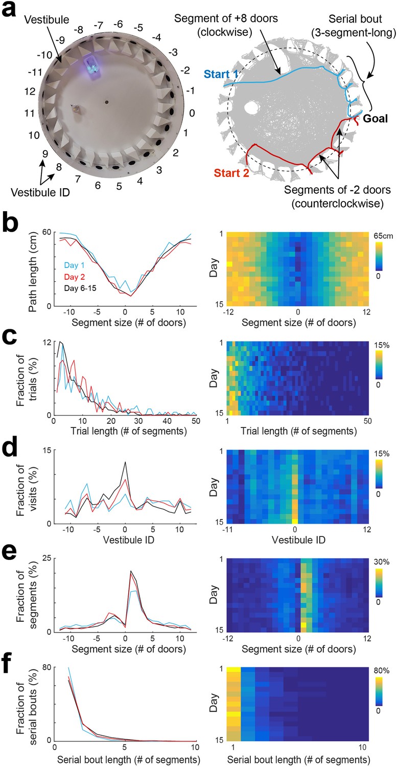
Statistical characterization of vestibule sequences across days.
(a) Top view of the maze (left) and two example trajectories on top of an overlay of multiple trajectories (right) showing vestibules and trajectory segmentation. The goal is at vestibule 0. Running segments span between two vestibule visits. Segment size is defined as the number of door-intervals a segment covers in the clockwise (positive sign) or counterclockwise (negative sign) direction. Serial bouts are bouts of consecutive 1-door-long segments. (b) The average path length as a function of segment size for 3 time periods capturing the dynamic range of the distributions (lines) and across days (color coded). (c–f) Same display as in (b) for the distribution of trial lengths (the number of segments per trial) (c), the distribution of visits across vestibules (d) (notice the peak at vestibule 0, which is the goal location), the distribution of segment sizes (e), and the distribution of serial bout lengths (f).
Figure 2—figure supplement 1
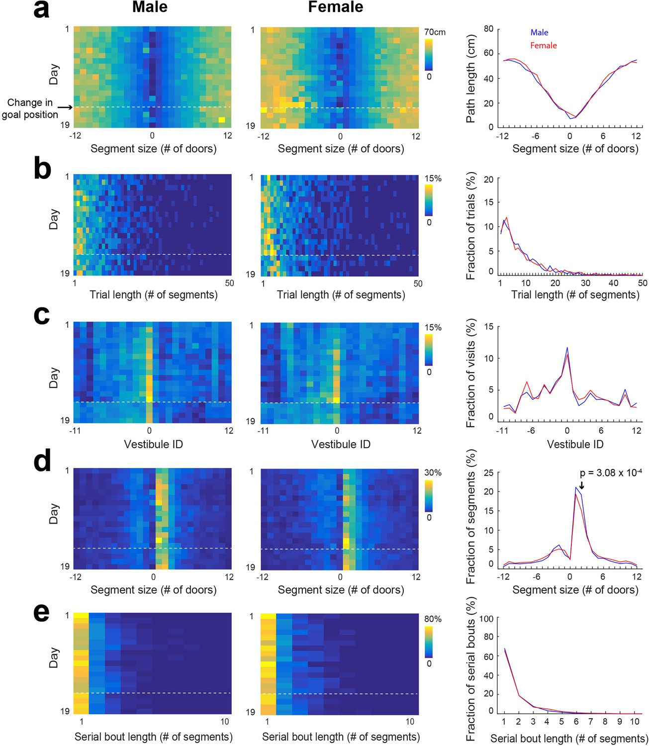
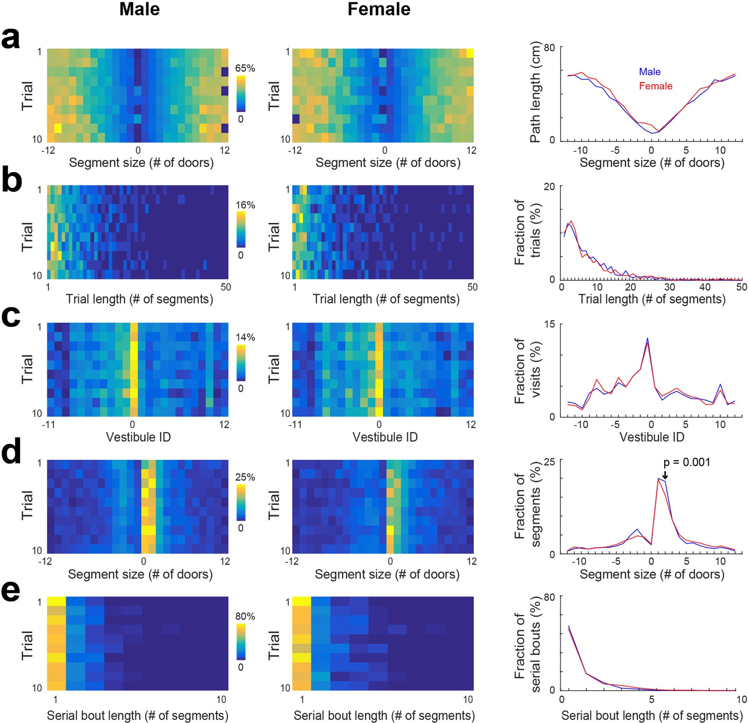
Statistical characterization of vestibule sequences across days, for male and female separately.
(a) The average path length as a function of segment size across the 15 training days and 4 reversal days (color coded) and averaged across day 6–15 (lines) for male and female separately. (b–e) Same display as in (a) for the distribution of trial lengths (the number of segments per trial) (b), the distribution of visits across vestibules (c), the distribution of segment sizes (d), and the distribution of serial bout lengths (e).
Figure 2—figure supplement 2
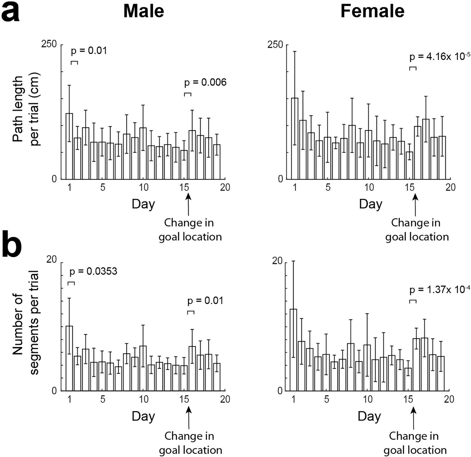
Path length and number of segments per trial across days.
(a) Average path length per trial across days, for male (left) and female (right). (b) Average number of segments per trial across days, for male (left) and female (right). (mean ± standard deviation, two-tailed paired t-test).
Figure 2—figure supplement 3
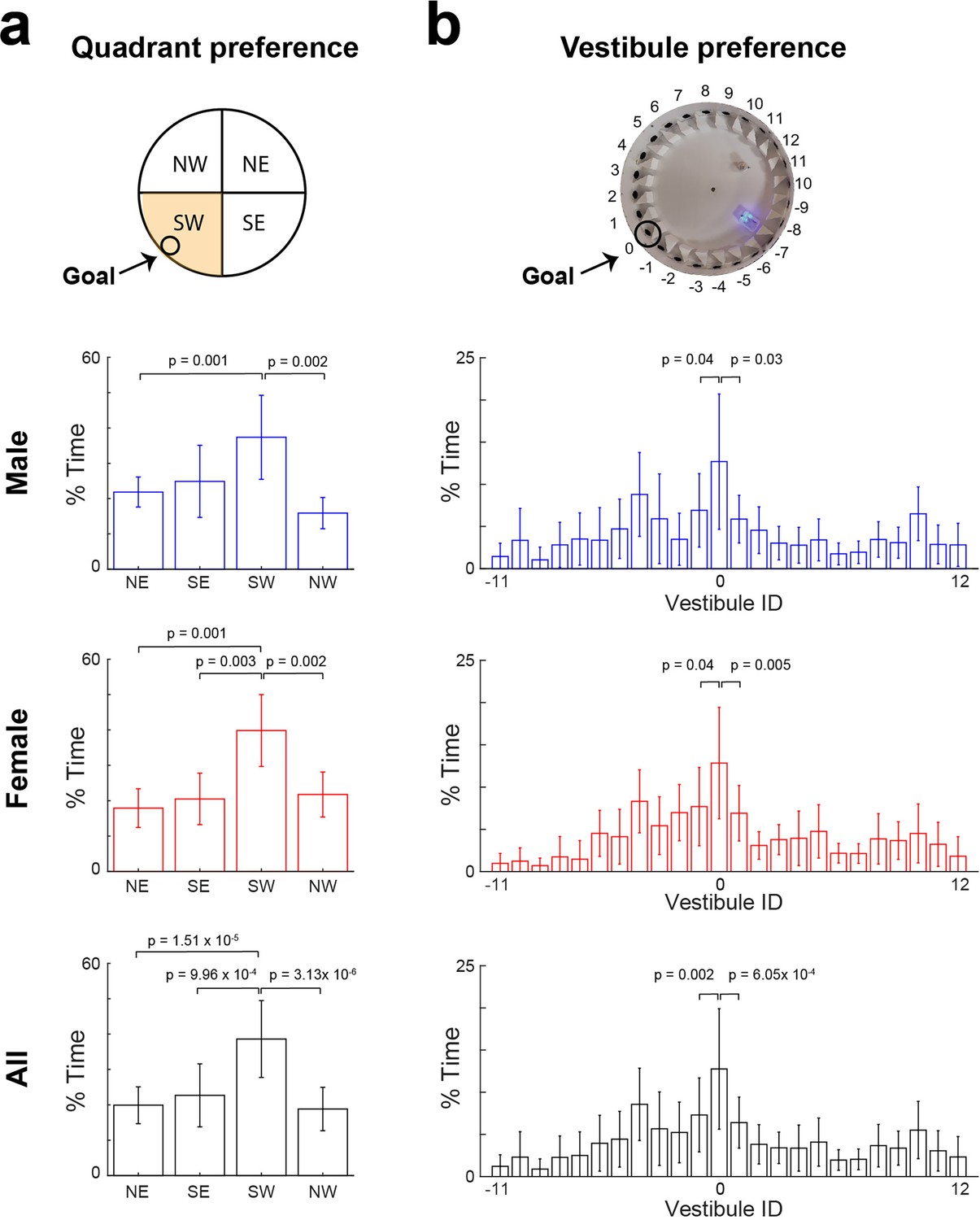
Quadrant and vestibule preference during the probe test.
(a) Fraction of time spent in each quadrant of the arena during the probe test, for male (blue), female (red), and all mice (black). (b) Fraction of time spent in each vestibule during the probe tests, for male (blue), female (red), and all mice (black). (mean ± standard deviation, two-tailed paired t-test).
Figure 2—figure supplement 4
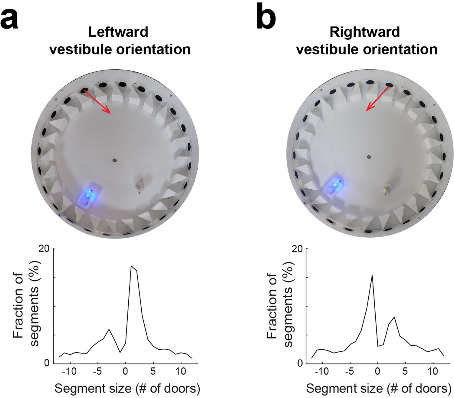
Vestibule orientation determines the direction of serial behavior.
(a) Top view of the arena (upper) and distribution of segment sizes (lower) for a leftward orientation of vestibules (red arrow). (b) Same as (a) for a rightward orientation of vestibules. Notice the reversal of the two peaks of the distributions, indicating that mice tend to visit consecutive vestibules via the clockwise (anti-clockwise) direction for the leftward (rightward) vestibule orientation.
Figure 3 with 1 supplement
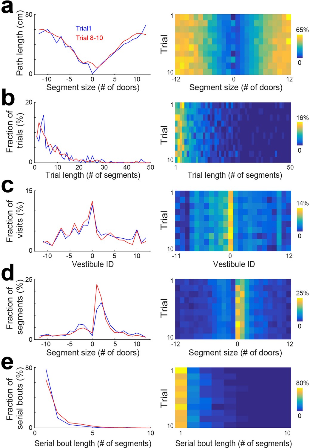
Statistical characterization of vestibule sequences across trials.
(a) The average path length as a function of segment size for 2 time periods capturing the dynamic range of the distributions (lines) and across trials (color coded). The data from days 6 to 15 were used for this analysis. (b–e) Same display as in (a) for the distribution of trial lengths (the number of segments per trial) (b), the distribution of visits across vestibules (c), the distribution of segment sizes (d), and the distribution of serial bout lengths (e).
Figure 3—figure supplement 1
Statistical characterization of vestibule sequences across trials, for male and female separately.
(a) The average path length as a function of segment size across trials (color coded) and averaged across trials (lines) for male and female separately. The data from days 6 to 15 were used for this analysis. (b–e) Same display as in (a) for the distribution of trial lengths (the number of segments per trial) (b), the distribution of visits across vestibules (c), the distribution of segment sizes (d), and the distribution of serial bout lengths (e).
Figure 4
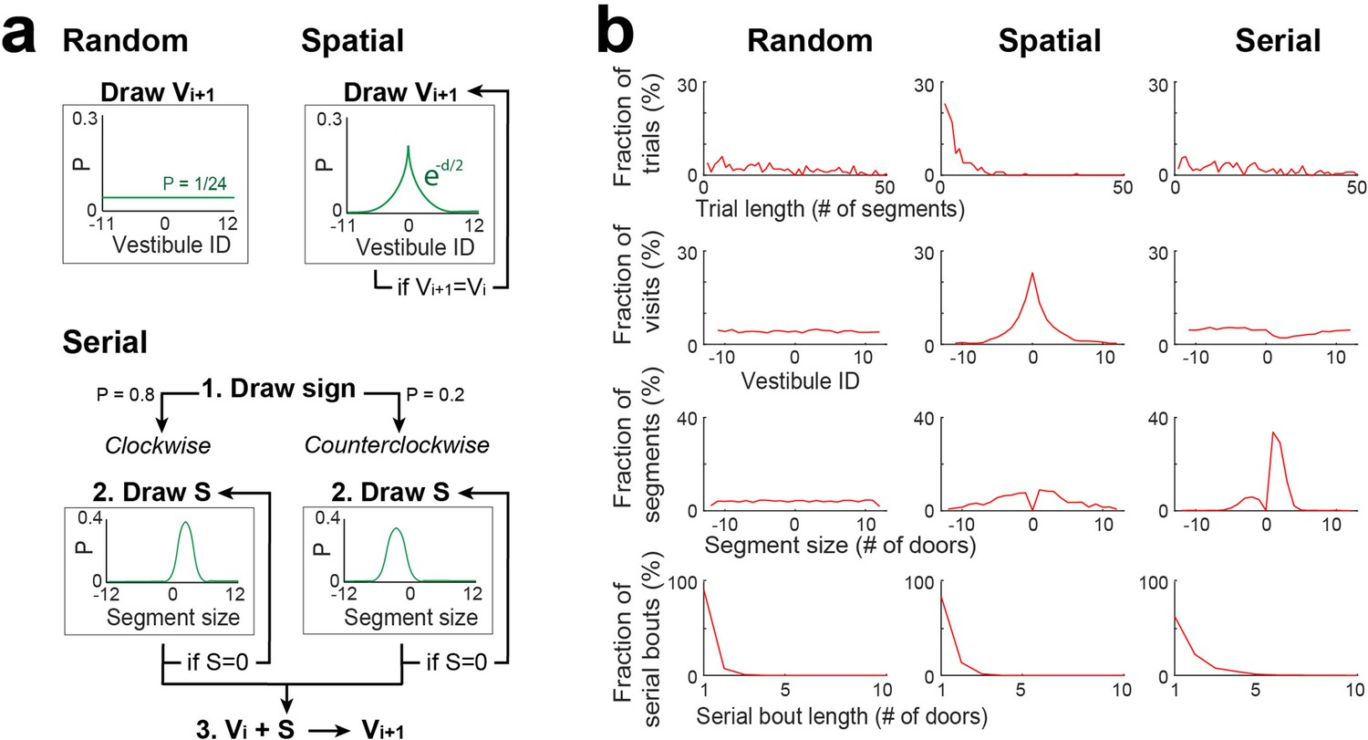
Stochastic processes for random, spatial and serial strategies.
(a) Schemes describing the stochastic processes for random, spatial and serial strategies. Vi +1: the next vestibule visited; Vi: the current vestibule; S: the next segment (a number of door-interval and a sign indicating clockwise/counterclockwise direction); and green lines: the probability distributions for random draws. Random strategy: Vi +1 is randomly drawn from the uniform distribution. Spatial strategy: Vi +1 is randomly drawn from a symmetric exponential distribution, and redrawn if Vi +1 = Vi. Serial strategy: The serial strategy can occur in either the clockwise or counterclockwise direction. The value of S is randomly drawn from a normal distribution with distinct center and width values for clockwise and counterclockwise directions, and is redrawn if S=0. Then Vi is incremented by S to obtain Vi +1. For the implementation of a single process combining both directions, the sign of S is first drawn with a 0.8/0.2 probability bias for positive/negative values, respectively. (b) The same analyses as in Figure 2c–f, carried on vestibule sequences outputted by each stochastic process over 10 trials and 20 mice. For each trial, the stochastic process was recursively run until Vi = 0. Note that none of the individual processes is reproducing the distributions of Figure 2.
Figure 5 with 2 supplements
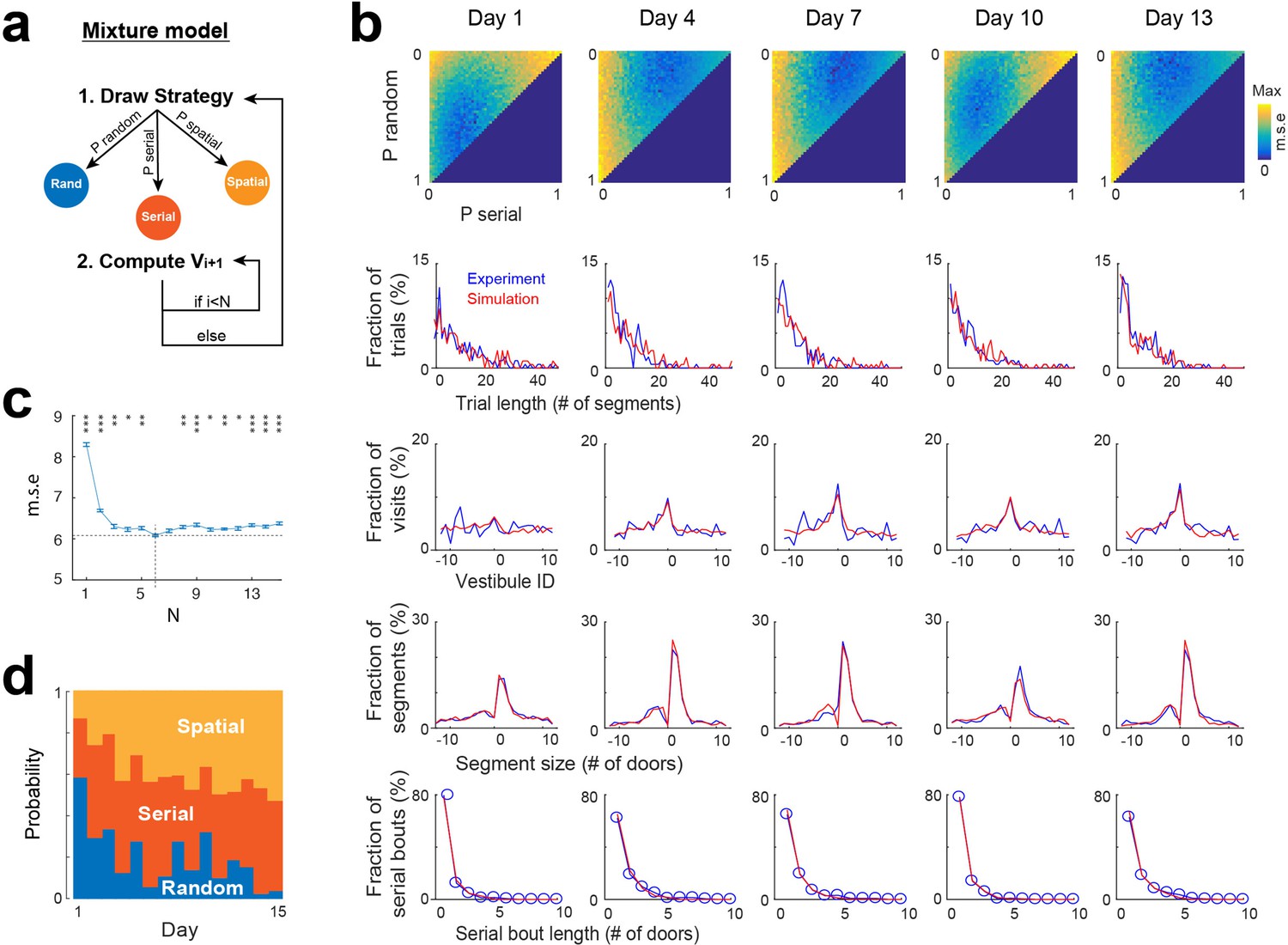
Mixture model fitting of strategy evolution across days.
(a) Mixture model combining the stochastic processes associated with random, spatial and serial strategies. A vestibule sequence is generated in two alternating steps. In step 1, a strategy is drawn according to the set of probabilities P_random, P_serial and P_spatial. In step 2, the stochastic process associated with the selected strategy is used to draw the next N vestibules. The vestibule sequence terminates upon reaching vestibule 0. Start positions are the same as in experiments. (b) Fits of experimental distributions for 5 days examples (using N=6). Color coded, mean square error (m.s.e) of the fits for all combinations of random, serial and spatial strategies (note that P_spatial = 1 P_random - P_serial). Line plots, overlays of experimental (blue) and model (red) distributions, for the best fits. (c) Mean square error as a function of N (mean ± s.e.m of 10 simulations for each value of N). A minimum is reached for N=6 (dash lines). Asterisks, significance relative to this minimum (*p<0.05, **p<0.005, ***p<0.0005, two-tail unpaired t-test). (d) Proportions of each strategy across days, obtained from the best fits.
Figure 5—figure supplement 1
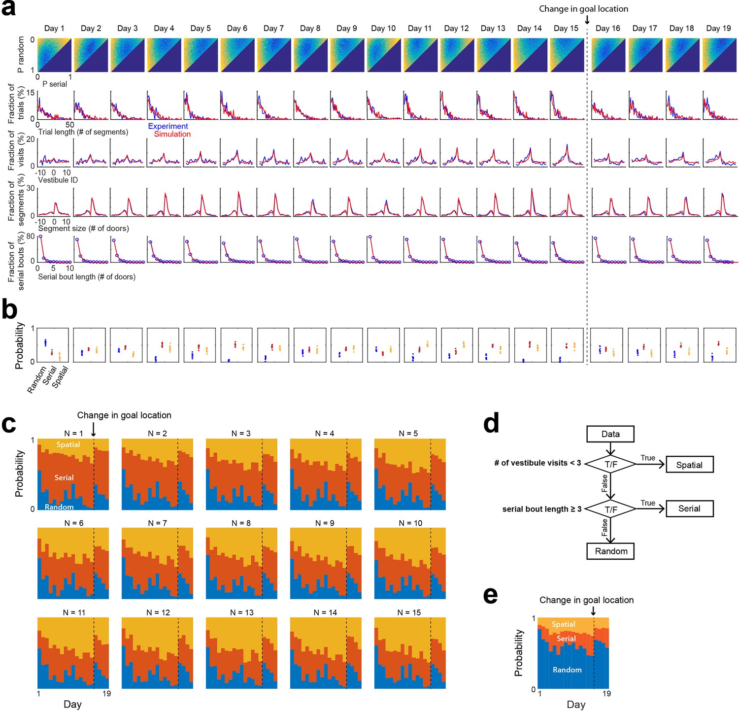
Strategy evolution across days based on the mixture model fit.
(a) Fits of experimental distributions across the 15 training days and 4 reversal days, using the mixture model and a strategy draw occurring every N=6 segments. Color coded, mean square error (m.s.e) between model and experimental distributions for all combinations of random, serial and spatial strategies (note that P_spatial = 1 P_random - P_serial). Line plots, overlays of experimental (blue) and model (red) distributions, for the best fits. (b) Proportions of each strategy across days, obtained from the model best fits, for 10 repetitions of the simulation with N=6. (c) Proportions of each strategy across days, obtained from the model best fits for various values of N. (d) Criteria previously used to classify strategies in the Barnes maze. Trials with less than 3 vestibule visits are assigned a spatial strategy. Trials for which the goal is reached via a serial bout at least 3-door-long are assigned a serial strategy. The rest of the trials are assigned a random strategy. (e) Proportions of each strategy across days, calculated with the criteria described in (d).
Figure 5—figure supplement 2
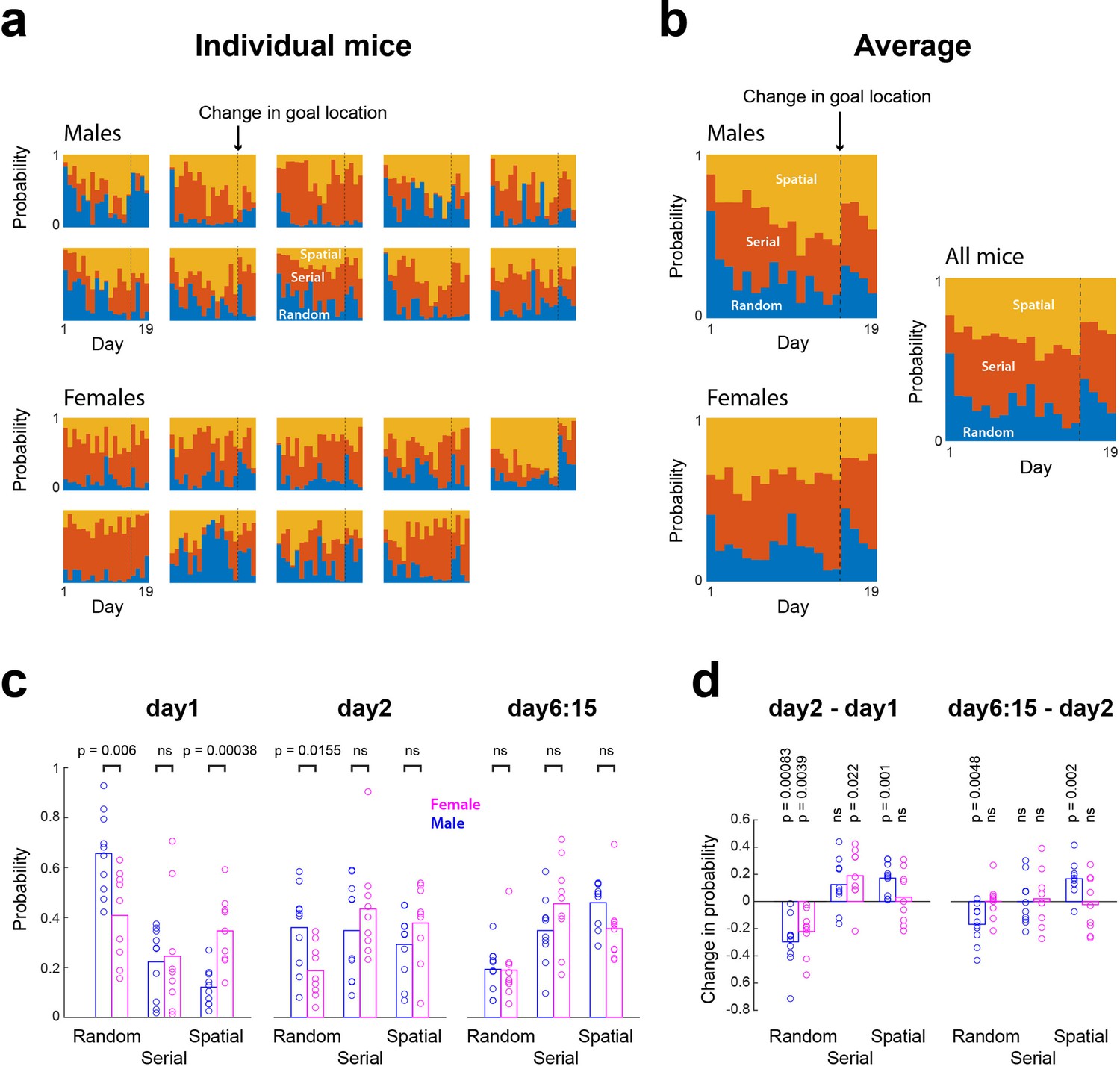
Inter-animal variations in search strategy across days.
(a) Proportions of each strategy across days for individual animal, obtained from the best fits of the mixture model. (b) Average proportions of each strategy across male (upper left), female (lower left) and all mice (right) (note the similarity with the proportions of each strategy obtained using the pooled data shown in Figure 5d). (c) Proportion of each strategy on day1, day2 and day6-to-15 combined (bar, mean; circle, individual mice; two-tailed unpaired t-test). (d) Initial (day2 - day1) and later (day6:15 day2) changes in strategy proportions (two-tailed t-test).
Figure 6
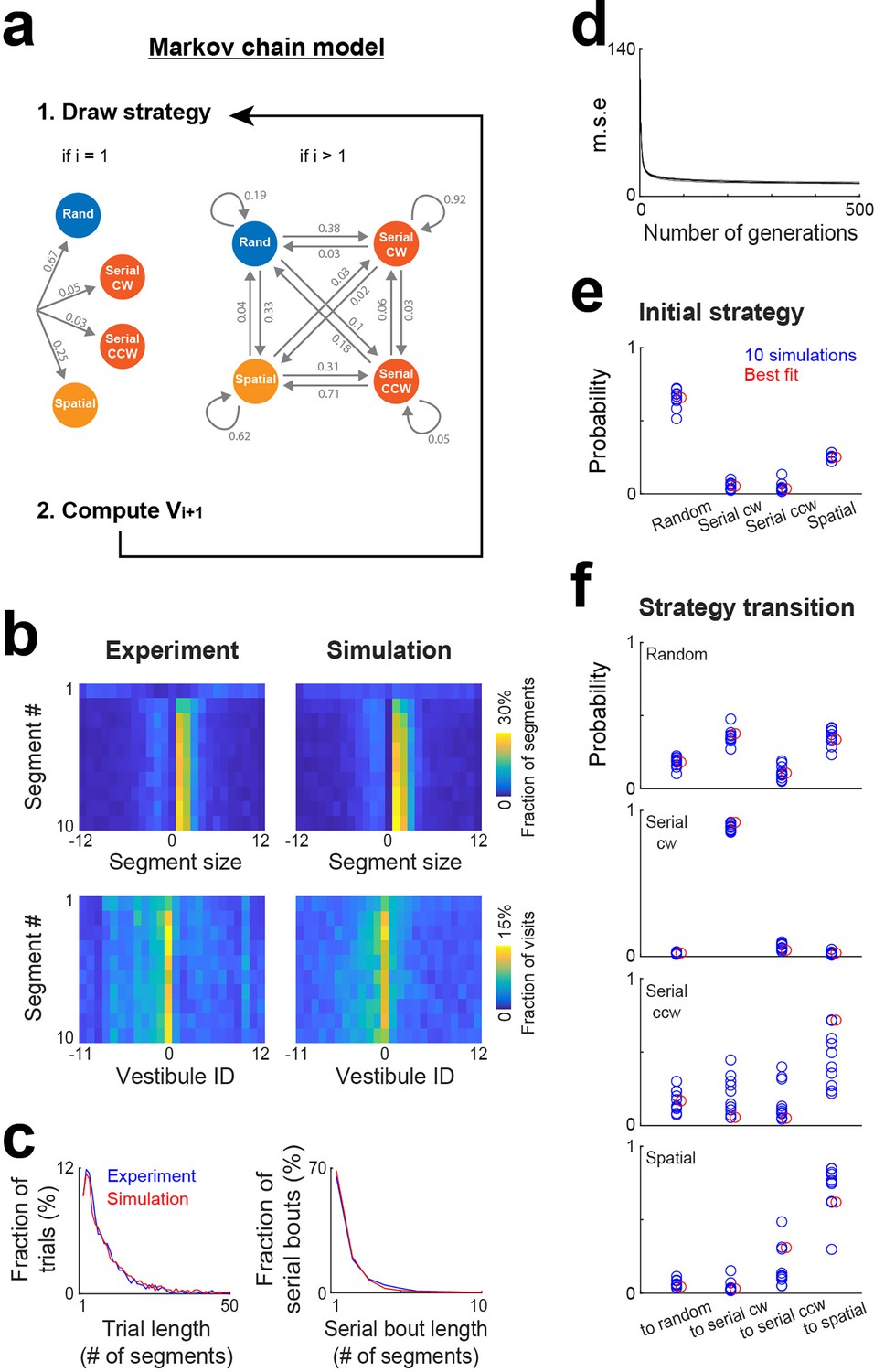
Markov chain modeling of within-trial strategy evolution.
(a) Markov chain model incorporating four strategies (random, serial clockwise, serial counterclockwise and spatial). To generate vestibule sequences, the model iteratively draws a strategy and then a vestibule using the stochastic process associated with the selected strategy, repeating this operation until the goal (vestibule 0) is reached. At the beginning of the trials (i=1), the strategy is drawn according to a set of probabilities determining the initial strategy. Subsequently (i>1), the model transitions between strategies based on another set of probabilities. Numbers indicate the probabilities obtained from the model best fit. (b) Experimental and model (best fit) distributions for segment size and vestibule visits, implemented on the level of individual segments for the first 10 segments of the trials. The data from days 6 to 15 were used for this analysis. (c) Overlays of experimental (blue) and model (red) distributions for both trial length and serial bout length, using the same fit instance as in (b). (d) Evolution of the mean square error (m.s.e) across generations of the genetic algorithm, for the 10 repetitions of the genetic algorithm. (e–f) Blue circles, set of probabilities determining the initial strategy (e) and strategy transitions (f), generated by 10 repetitions of the genetic algorithm. Red circles, the probability set that produced the smallest m.s.e.
Additional files
Download links
A two-part list of links to download the article, or parts of the article, in various formats.
Downloads (link to download the article as PDF)
Open citations (links to open the citations from this article in various online reference manager services)
Cite this article (links to download the citations from this article in formats compatible with various reference manager tools)
Stochastic characterization of navigation strategies in an automated variant of the Barnes maze
eLife 12:RP88648.
https://doi.org/10.7554/eLife.88648.4


