When and why does motor preparation arise in recurrent neural network models of motor control?
- Computational and Biological Learning Lab, Department of Engineering, University of Cambridge, United Kingdom
- Meta Reality Labs, United States
Figures
Figure 1
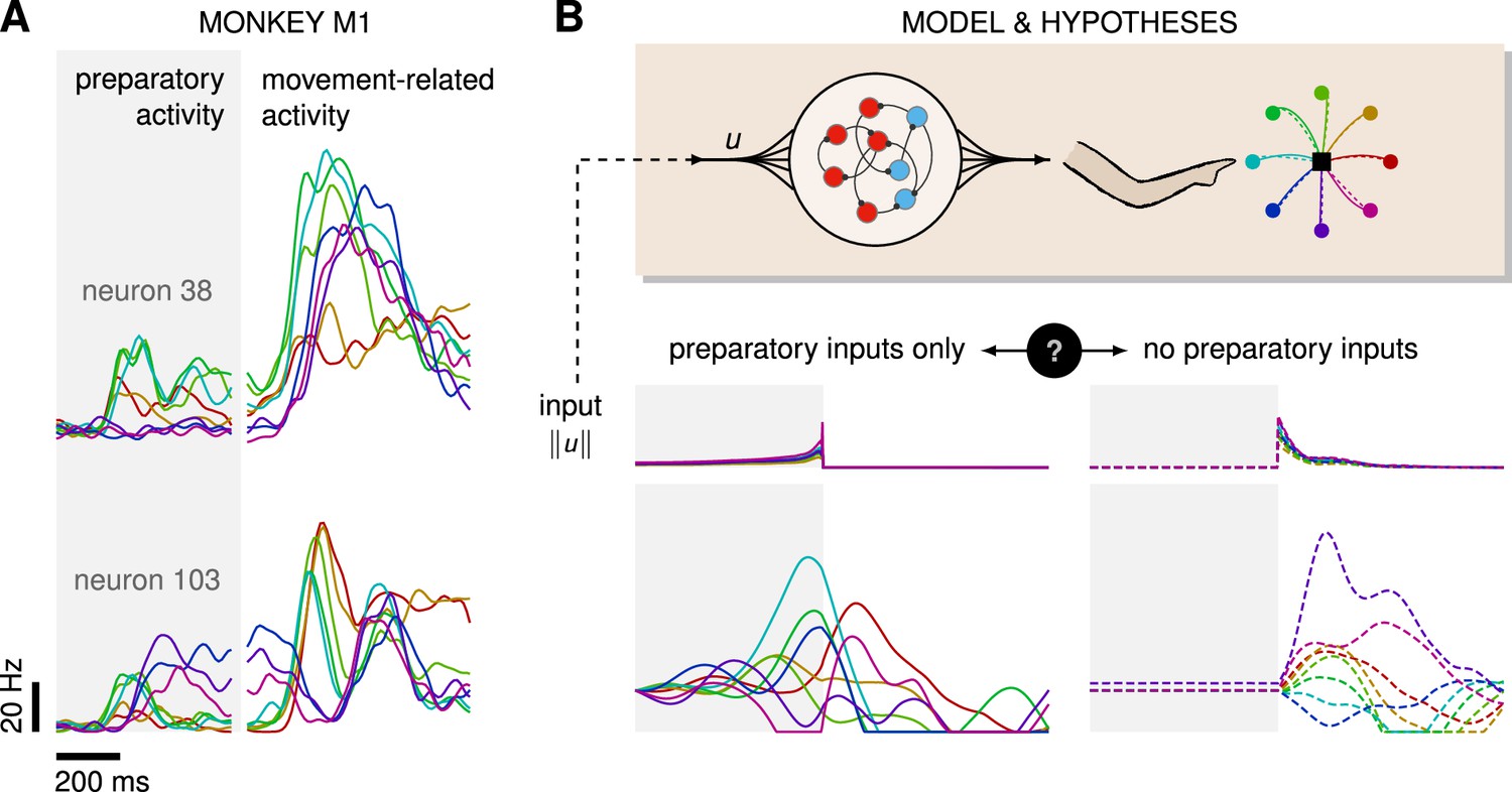
Control is possible under different strategies.
(A) Trial-averaged firing rate of two representative monkey primary motor cortex (M1) neurons, across eight different movements, separately aligned to target onset (left) and movement onset (right). Neural activity starts separating across movements well before the animal starts moving. (B) Top: a recurrent neural network (RNN) model of M1 dynamics receives external inputs from a higher-level controller, and outputs control signals for a biophysical two-jointed arm model. Inputs are optimized for the correct production of eight center-out reaches to targets regularly positioned around a circle. Bottom: firing rate of a representative neuron in the RNN model for each reach, under two extreme control strategies. In the first strategy (left, solid lines), the external inputs are optimized while being temporally confined to the preparatory period. In the second strategy (right, dashed lines), they are optimized while confined to the movement period. Although slight differences in hand kinematics can be seen (compare corresponding solid and dashed hand trajectories), both control policies lead to successful reaches. These introductory simulations are shown for illustration purposes; the particular choice of network connectivity and the way the control inputs were found are described in the Results section.
Figure 2
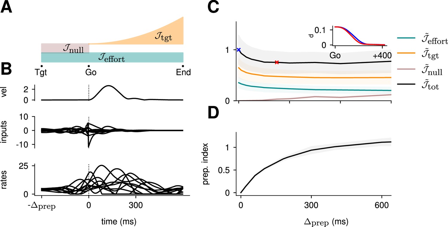
Optimal control of the inhibition-stabilized network (ISN).
(A) Illustration of the different terms in the control cost function, designed to capture the different requirements of the task. ‘Tgt’ marks the time of target onset, ‘Go’ that of the go cue (known in advance), and ‘End’ the end of the trial. (B) Time course of the hand velocity (top), optimal control inputs (middle; 10 example neurons), and firing rates (bottom, same neurons) during a delayed reach to one of the eight targets shown in Figure 1A. Here, the delay period was set to ms. Note that inputs arise well before the go cue, even though they have no direct effect on behavior at that stage. (C) Dependence of the different terms of the cost function on preparation time. All costs are normalized by the total cost at ms. The inset shows the time course of the hand’s average distance to the relevant target when no preparation is allowed (blue) and when preparation is allowed (red). Although the target is eventually reached for all values of , the hand gets there faster with longer preparation times, causing a decrease in – and therefore also in . Another part of the decrease in is due to a progressively lower input energy cost . On the other hand, the cost of staying still before the go cue increases slightly with . (D) We define the preparation index as the ratio of the norms of the external inputs during preparation and during movement (see text). The preparation index measures how much the optimal strategy relies on the preparatory period. As more preparation time is allowed, this is used by the optimal controller and more inputs are given during preparation. For longer preparation times, this ratio increases sub-linearly, and eventually settles.
Figure 3
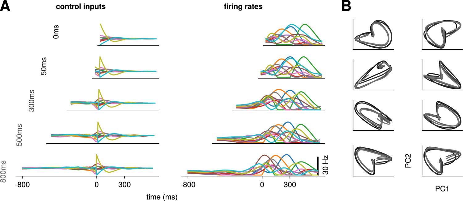
Conservation of the optimal control strategy across delays.
(A) Optimal control inputs to 10 randomly chosen neurons in the model recurrent neural network (RNN) (left) and their corresponding firing rates (right) for different preparation times (ranging from 0 to 800 ms; c.f. labels). (B) Projection of the movement-epoch population activity for each of the eight reaches (panels) and each value of shown in A (darker to lighter colors). These population trajectories are broadly conserved across delay times, and become more similar for larger delays.
Figure 4
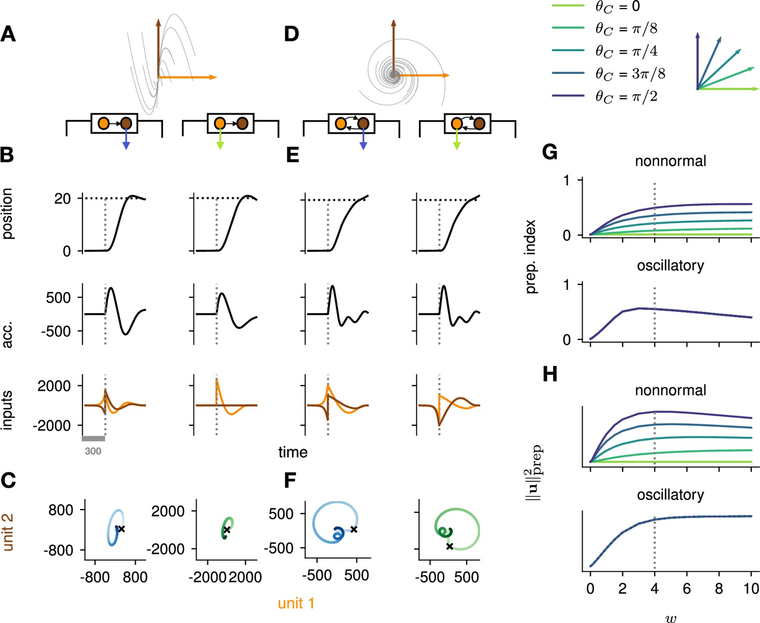
Analysis of the interplay between the optimal control strategy and two canonical motifs of E-I network dynamics: nonnormal transients driven by feedforward connectivity (A–C), and oscillations driven by anti-symmetric connectivity (D–F).
(A) Activity flow field (10 example trajectories) of the nonnormal network, in which a ‘source’ unit (orange) drives a ‘sink’ unit (brown). We consider two opposite readout configurations, where it is either the sink (left) or the source (right) that drives the acceleration of the hand. (B) Temporal evolution of the hand position (top; the dashed horizontal line indicates the reach target), hand acceleration (middle), and optimal control inputs to the two units (bottom; colors matching panel A), under optimal control given each of the two readout configurations shown in A (left vs. right). The dashed vertical line marks the go cue, and the gray bar indicates the delay period. While the task can be solved successfully in both cases, preparatory inputs are only useful when the sink is read out. (C) Network activity trajectories under optimal control. Each trajectory begins at the origin, and the end of the delay period is shown with a black cross. (D–F) Same as (A–C), for the oscillatory network. (G–H) Preparation index (top) and total amount of preparatory inputs (bottom) as a function of the scale parameter of the network connectivity, for various readout configurations (color-coded as shown in the top inset). The nonnormal network (top) prepares more when the readout is aligned to the most controllable mode, while the amount of preparation in the oscillatory network (bottom) is independent of the readout direction. The optimal strategy must balance the benefits from preparatory inputs which allow to exploit the intrinsic network dynamics, with the constraint to remain still. This is more difficult when the network dynamics are strong and pushing activity out of the readout-null subspace, explaining the decrease in preparation index for large values of in the oscillatory network.
Figure 5
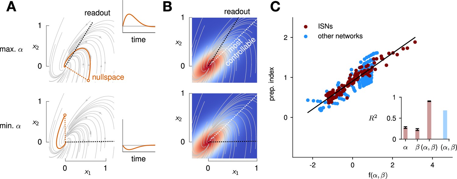
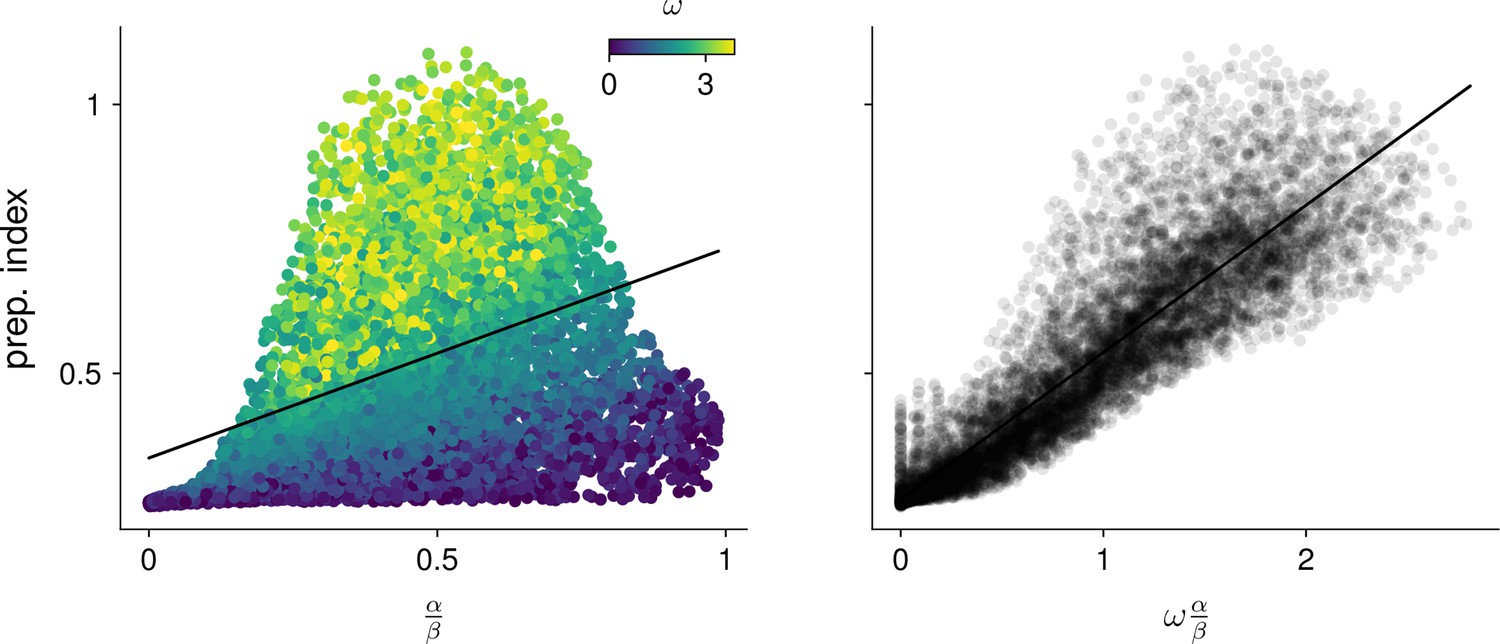
Predicting the preparation index from the observability of the output nullspace (α) and the controllability of the readout (β, see details in text).
(A) Illustration of the observability of the output nullspace in a synthetic two-dimensional system. The observability of a direction is characterized by how much activity (integrated squared norm) is generated along the readout by a unit-norm initial condition aligned with that direction. The top and bottom panels show the choices of readout directions (dotted black) for which the corresponding nullspace (dotted orange) is most (maximum α) and least (minimum α) observable, respectively. Trajectories initialized along the null direction are shown in solid orange, and their projections onto the readout are shown in the inset. (B) Illustration of the controllability of the readout in the same 2D system as in (A). To compute controllability, the distribution of activity patterns collected along randomly initialized trajectories is estimated (heatmap); the controllability of a given direction then corresponds to how much variance it captures in this distribution. Here, the network has a natural propensity to generate activity patterns aligned with the dashed white line (‘most controllable’ direction). The readout directions are repeated from panel A (dotted black). The largest (resp. smallest) value of β would by definition be obtained when the readout is most (resp. least) controllable. Note the tradeoff in this example: the choice of readout that maximizes α (top) does not lead to the smallest β. (C) The values of α and β accurately predict the preparation index () for a range of high-dimensional inhibition-stabilized networks (ISNs) (maroon dots) with different connectivity strengths and characteristic timescales (Methods). The best fit (after z-scoring) is given by (mean ± s.e.m. were evaluated by boostrapping). This confirms our hypothesis that optimal control relies more on preparation when is large and β is small. Note that α and β alone only account for 34.8% and 30.4% of the variance in the preparation index, respectively (inset). Thus, α and β provide largely complementary information about the networks’ ability to use inputs, and can be combined into a very good predictor of the preparation index. Importantly, even though this fit was obtained using ISNs only, it still captures 69% of preparation index variance across networks from other families (blue dots; Methods).
Figure 6
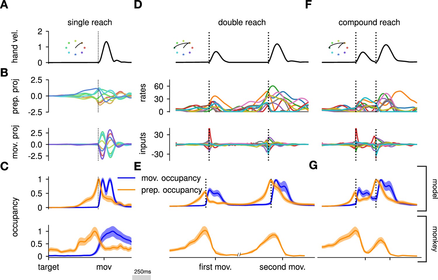
The model executes a sequence of two reaches using an independent strategy.
(A) Hand velocity during one of the reaches, with the corresponding hand trajectory shown in the inset. (B–C) We identified two six-dimensional orthogonal subspaces, capturing 79% and 85% of total activity variance during single-reach preparation and movement respectively. (B) First principal component of the model activity for the eight different reaches projected into the subspaces identified using preparatory (top) and movement-epoch (bottom) activity. (C) Occupancy (total variance captured across movements) of the orthogonalized preparatory and movement subspaces, in the model (top) and in monkey motor cortical activity (bottom; reproduced from Lara et al., 2018, for monkey Ax). We report mean ± s.e.m., where the error is computed by bootstrapping from the neural population as in Lara et al., 2018. We normalize each curve separately to have a maximum mean value of 1. To align the model and monkey temporally, we re-defined the model’s ‘movement onset’ time to be 120 ms after the model’s hand velocity crossed a threshold – this accounts for cortico-spinal delays and muscle inertia in the monkey. Consistent with Lara et al., 2018’s monkey primary motor cortex (M1) recordings, preparatory subspace occupancy in the model peaks shortly before movement onset, rapidly dropping thereafter to give way to pronounced occupancy of the movement subspace. Conversely, there is little movement subspace occupancy during preparation. (D) Behavioral (top) and neural (middle) correlates of the delayed reach for one example of a double reach with an enforced pause of 0.6 s. The optimal strategy relies on preparatory inputs preceding each movement. (E) Same as (C), for double reaches. The onsets of the monkey’s two reaches are separately aligned to the model’s using the same convention as in (C). The preparatory subspace displays two clear peaks of occupancy. This double occupancy peak is also observed in monkey neural activity (bottom; reproduced from Zimnik and Churchland, 2021, with the first occupancy peak aligned to that of the model). (F) Same as (D), for compound reaches with no enforced pause in-between. Even though the sequence could be viewed as a single long movement, the control strategy relies on two periods of preparation. Here, inputs before the second reach are used to reinject energy into the system after slowing down at the end of the first reach. (G) Even though no explicit delay period is enforced in-between reaches during the compound movement, the preparatory occupancy rises twice, before the first reach and once again before the second reach. This is similar to observations in neural data (bottom; reproduced from Zimnik and Churchland, 2021).
Appendix 1—figure 1
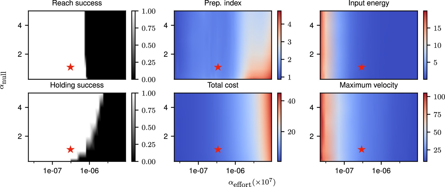
Correlates of the behavior and control strategy across a wide range of hyperparameters.
The ‘reach success’” and ‘holding success’” are set to 1 if the success criterion (see text) is satisfied and 0 otherwise. The task is executed successfully over a wide range of hyperparameters. The red star denotes the set of hyperparameters used in the main text simulations. This configuration was chosen to lie in a region in which the task can be successfully solved, with the performance being robust to small changes in the hyperparameters.
Appendix 1—figure 2
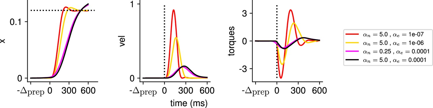
Illustration of the behavior for several hyperparameter settings.
(Left) Hand position along the horizontal axis, with the dotted line denoting the position of the target. (Middle) Temporal profile of the hand velocity. (Right) Temporal profile of the torques driving the hand.
Appendix 1—figure 3

Illustration of the effect of the characteristic neuronal timescale on the temporal distribution of the inputs.
We modified the characteristic neuronal timescale of the inhibition-stabilized network (ISN) during preparation only and assessed how that changed the temporal distribution of inputs for three different timescales (τprep = 50 ms, τprep = 150 ms, τprep = 300 ms, top to bottom). As hypothesized, inputs start earlier during the preparation window when the decay timescale of the network was longer.
Appendix 1—figure 4

Illustration of α and β as a function of θC and w in the 2D networks.
Appendix 1—figure 5
Predicting the preparation index from characteristic network quantities.
We evaluated how well the preparation index could be predicted as a linear function of (left). A substantial amount of residual variance appeared to arise from variability in the oscillation frequency (color). Accounting for this frequency by regressing the preparation index against gave a better fit (right).
Appendix 1—figure 6
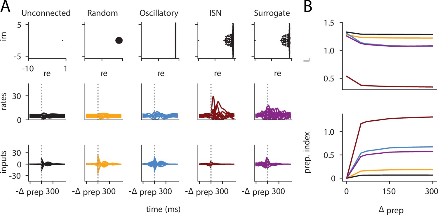
Preparation arises across a range of network architectures: neural correlates of the reach are shown for five different networks (A), alongside the loss and prep.
index as a function of . (A) Eigenvalue spectrum (top), internal network activations (middle), and inputs (bottom) for different network types. The unconnected network does not rely on preparatory inputs at all. The random network with weights draw from uses very little delay-period inputs while the skew-symmetric network with shows a substantial amount of inputs during the delay period. The inhibition-stabilized network can be seen to rely most on preparation, more so than the similarity transformed inhibition-stabilized network (ISN). (B) Loss (top) and preparation index (bottom) as a function of delay-period length for the different networks. The unconnected and random networks can be seen to benefit very little from longer preparation times. Indeed, even as increases, their amount of preparatory inputs remains very close to 0. On the other hand, the skew-symmetric network and the ISN use preparatory inputs (bottom), which allow them to have a lower loss for larger values of . Interestingly, the surrogate ISN prepares considerably less than the full ISN.
Appendix 1—figure 7
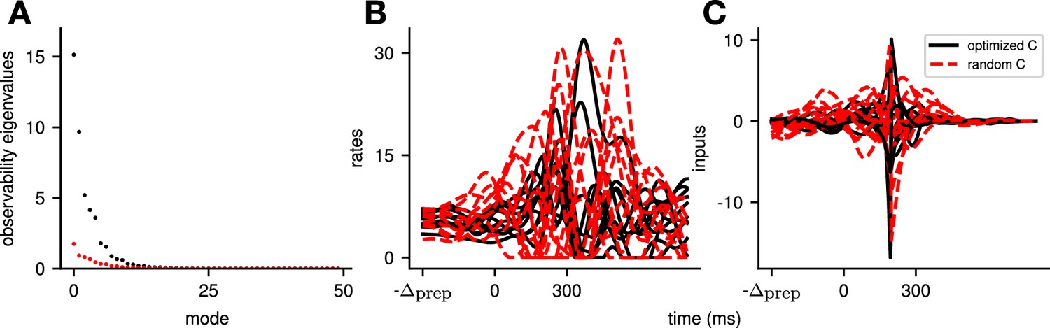
Illustration of the effect of optimizing the readout matrix such as to minimize the cost of the reaches, across all movements.
To evaluate the effect that our choice of random readout directions has on our conclusions, we additionally compare to a model with the same dynamics, but where the readout was optimized such as to minimize the cost across movements (i.e. ), under the constraint that its norm was fixed. In (A), we see that this leads to an increase in the observability of the system (compare the observability of the modes of the optimized system in black with those of the random readout in red). In (B) and (C), we see that this leads to an output of similar amplitude (B), but that is generated using smaller inputs (C). Importantly, we see that the system still relies on preparatory inputs. Thus, the exact choice of readout does not alter the network strategy, but can help the system perform the same movements in a more efficient manner.
Appendix 1—figure 8
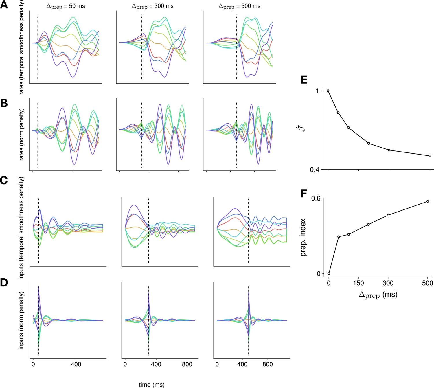
Comparison of the effect of penalizing temporal input smoothness vs. input norm.
We compare the effect of using a cost over inputs that penalizes input norm, vs. using a cost that penalizes the ‘temporal complexity’ of the inputs – defined here as the temporal derivative of the inputs (i.e. in discrete time). This is achieved by augmenting the dynamical system to include an input integration stage, which then feeds into the original dynamical system; this way, the input to the augmented system – of which we continue to penalize the squared norm to enable the iterative linear quadratic regulator algorithm (iLQR) framework – is the derivative of the input to the original system. We perform this comparison in linear recurrent neural networks (RNNs), across a range of different preparation times. We show the activation of an example neuron in (A) and (B), and activity in an example input channel in (C) and (D). Each color denotes a different reach. We see that the rates vary more slowly when penalizing the temporal complexity (A) vs. the input norm (B), exhibiting a plateau for longer preparation times that is more similar to neural recordings. This is a reflection of the fact that the inputs themselves vary more slowly when the temporal complexity is penalized (compare C and D). As we do not penalize the input norm within our definition of temporal complexity, the optimal strategy is for the network to rely on steady inputs, which is different from the strategy used when the norm is penalized (compare C and D). We note that, under this different choice of input penalty, preparation nevertheless remains optimal, with the normalized loss (shown in E) decreasing as increases, and the preparation index (shown in F) increasing as increases.
Appendix 1—figure 9

Control strategy adopted by the model when planning with uncertain delays.
We investigate an extension of the model, that includes uncertainty about the arrival of the go cue, and involves replanning at regular intervals to update the model with new information (e.g. whether the go cue has arrived). In (A), we model this by assuming that the network is adopting a strategy whereby it plans to be ready to move as early as possible following the target onset. We optimize the inputs using this assumption, and replan every 20 ms to update the model with the available information (which here corresponds to the actual go cue only arriving 500 ms after target onset). We plot the activity of two example neurons (left and right panels, respectively), for each of the reaches (each color denotes a different reach). We can see that the neuronal activations start ramping up at the beginning of the task, and plateau before the actual target onset. In (B), we use a similar optimization strategy, but use a different ‘mental model’ for the network, whereby we assume that, until it sees the actual go cue, the model is always assuming that the delay period will be equal to the most likely a posteriori preparation time. Under the assumption of exponentially distributed delays with a mean of 150 ms, this corresponds to always replanning assuming a delay of 150 ms. We see that the network then adopts a different strategy, which does not include ramping/plateauing of the neural activity.
Appendix 1—figure 10
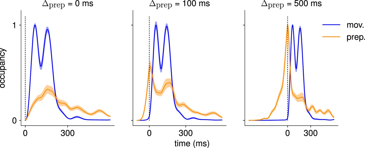
Comparison of the occupancy of the preparatory and movement subspaces across different delay periods.
Occupancy (normalized by the maximum value across preparatory and movement occupancies) of the preparatory and movement subspaces identified using a delay period of 500 ms, for the activity generated using ms (left), ms (center), and ms (right). We see that the network does not rely on preparatory activity when ms.
Additional files
Download links
A two-part list of links to download the article, or parts of the article, in various formats.
Downloads (link to download the article as PDF)
Open citations (links to open the citations from this article in various online reference manager services)
Cite this article (links to download the citations from this article in formats compatible with various reference manager tools)
When and why does motor preparation arise in recurrent neural network models of motor control?
eLife 12:RP89131.
https://doi.org/10.7554/eLife.89131.4


