Figures and data in Dynamical mechanisms of growth-feedback effects on adaptive gene circuits | eLife

Figures
Additional files

15 figures and 1 additional file

Figures

Figure 1

Download asset Open asset

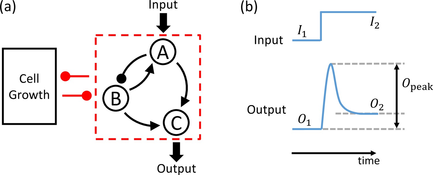
Schematic illustration of a synthetic adaptive gene circuit embedded in a host cell.

(a) A representative three-gene circuit (inside the dashed red box) and its dynamical interplay with host-cell growth. Arrows with triangular ends and round ends denote activating and inhibiting regulations, respectively. Altogether, there are 16,038 possible three-node topologies, with 425 topologies capable of adaptation. (b) An example of the circuit input and output signals. The input is an idealized step function of currents $I_{1}$ and $I_{2}$ before and after the jump, respectively. The output signal is a response of the circuit to the step function. The features of the output signal, as characterized by three key quantities characterizing the signal: $O_{1}$ , $O_{2}$ , and $O_{p e a k}$ , can be used to determine if the circuit has succeeded or failed in its intended function.

Figure 2

Download asset Open asset

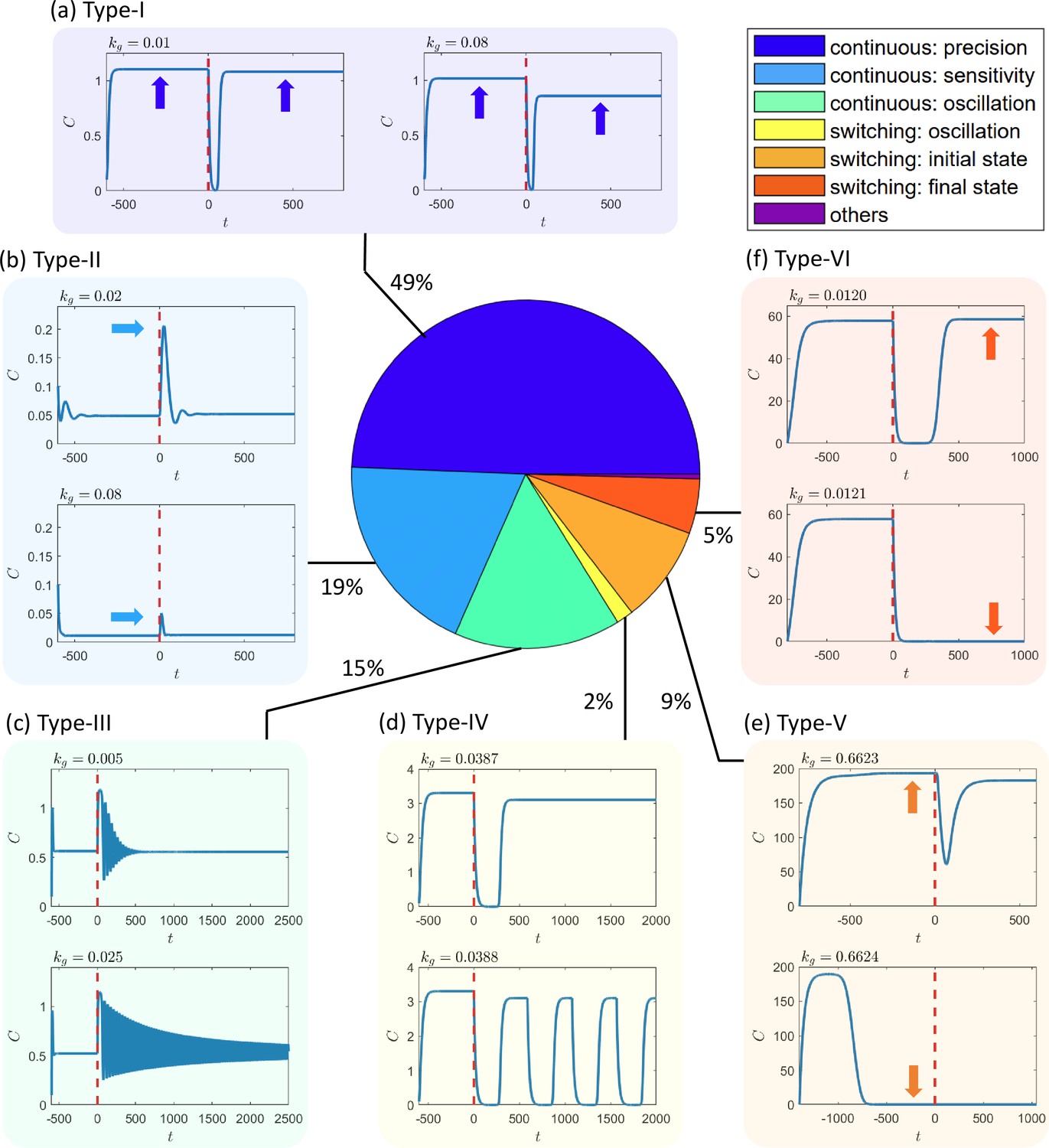
Systemic classification of circuit failure scenarios due to growth feedback.

This study identifies six computationally detectable categories of failures based on the criterion of functional adaptation that the circuit violates as the effect of growth feedback becomes stronger. (a) Type-I and (b) type-II failures correspond to the cases where the precision criterion or sensitivity criterion is violated in a continuous fashion as the growth-feedback strength $k_{g}$ increases, respectively. (c) Type-III and (d) type-IV failures occur when the circuits lose adaptation due to growth-feedback-induced oscillation, either continuously or abruptly, as $k_{g}$ increases, respectively. The abrupt changes in type-IV are caused by bifurcations, mostly a saddle-node bifurcation of cycles or an infinite-period bifurcation. For instance, the case shown in (d) undergoes an infinite-period bifurcation. (e) Type-V and (f) type-VI failures are when the circuits lose adaptation due to an abrupt change in $O_{1}$ or $O_{2}$ as $k_{g}$ increases, respectively, which are caused by bistability or multistability in the systems. Trials that are not categorized under these six classifications or fall into multiple categories constitute less than 0.4% of all cases (see text for more details and discussions about each failure class). The insets around the pie chart provide exemplary response curves of the circuits in each failure scenario. Each inset shows the concentration of the output node $C$ versus time with two values of the growth-feedback strength $k_{g}$ , one below and another above the failure threshold, for the specific failure scenario. In each case, the input is switched from state $I_{1}$ to $I_{2}$ at the time indicated by the red vertical dashed line.

Figure 3

Download asset Open asset

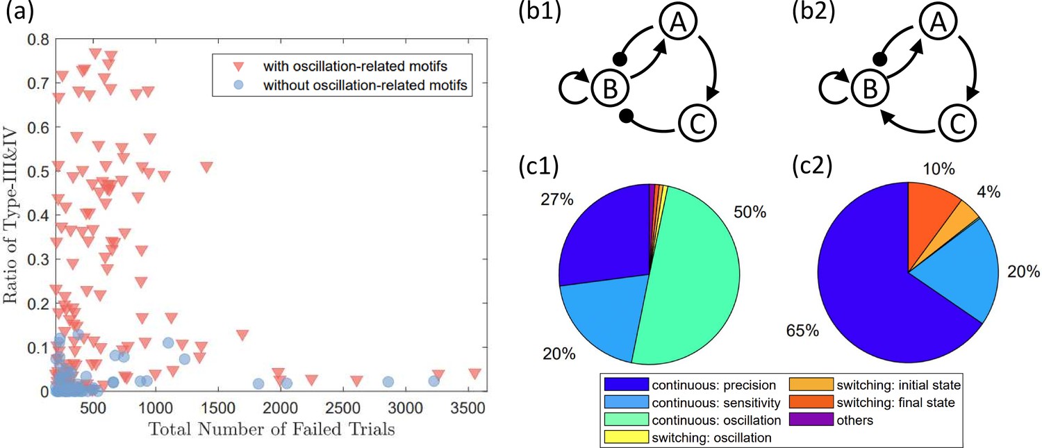
Fractions of growth-feedback-induced oscillation failures for different network topologies.

(a) There are significant variations across network topologies in the fraction of circuit failures attributable to growth-feedback-induced oscillations (types III and IV). Some topologies exhibit virtually no oscillation-related malfunctions, while others experience about 80% of failures caused by growth-induced oscillations. Network topologies containing any oscillation-supporting motifs (discussed in the main text) are represented by red triangles, while the rest are shown as blue circles. The majority of red data points have higher fractions of oscillation-related failures compared to the blue ones, mainly due to the presence of oscillation-supporting motifs. To reduce fluctuations in the results, only circuit topologies with over 200 failed trials are included. (b1, b2) A pair of network topologies that differ by only one link (from node C to B). (c1, c2) The distinct topologies in (b1, b2) leading to different distributions of failure mechanisms. The topology in (b1) primarily experiences growth-induced oscillation as the major failure mechanism, while the one in (b2) has barely any trials with growth-feedback-induced oscillations.

Figure 4

Download asset Open asset

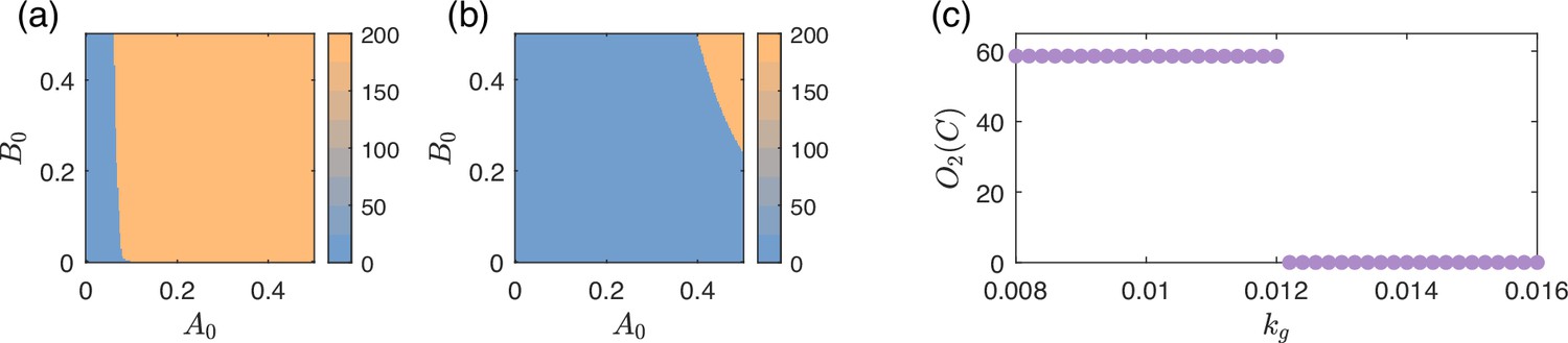
Bistability behind both the type-V and type-VI failures.

(a, b) Basin structure of the circuit shown in Figure 2e (with type-V failure) for input $I_{1}$ with different levels of growth feedback, for growth-feedback strength $k_{g} = 0.05$ (weak) and $k_{g} = 0.97$ (relatively strong). The coordinates $A_{0}$ and $B_{0}$ are the initial values of nodes A and B, respectively, corresponding to a two-dimensional slice of the entire four-dimensional phase space by fixing $C = 0.1$ and $N = 10^{- 3}$ . The color bar indicates the equilibrium value of node C before the input switch, which is $O_{1} (C)$ . There is bistability in both cases, as there are two basins of attraction. The yellow region is the functional basin that has adaptation, while the blue region is a non-functional basin without adaptation. The relative size of the blue non-functional region with larger $k_{g}$ in this case is significantly larger and includes the initial state of the system ( $A_{0} = B_{0} = 0.1$ ), causing a type-V circuit failure. (c) Diagram of $O_{2} (C)$ from the circuit in Figure 2f with a type-VI failure. Prior to a threshold value of $k_{g} \approx 0.012$ , one higher stable value of $O_{2} (C)$ exists. After this threshold, the state suddenly switches to a lower $O_{2} (C)$ one. Note that this abrupt change is not caused by a bifurcation. Instead, it is caused by $O_{1}$ continuously changing with respect to $k_{g}$ crossing a basin boundary of $O_{2}$ .

Figure 5

Download asset Open asset

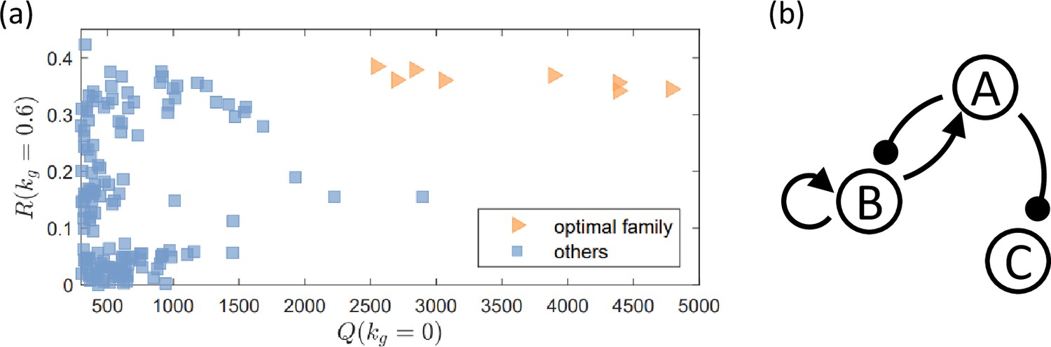
A family of circuit topologies with optimal performance.

The circuits both have a large volume of the functional region in the parameter space in the absence of growth feedback as characterized by a large value of $Q (k_{g} = 0)$ and are robust against growth feedback with a high value of $R (k_{g})$ . (a) Values of $Q (k_{g} = 0)$ and $R (k_{g} = 0.6)$ from all the 425 network topologies, where each data point corresponds to a topology. The family of optimal topologies is represented by the orange data points, including eight network topologies. (b) The set of links (motif) shared by this family of circuits. The combination of these links is also one of the minimal topologies with perfect adaptation in three regulatory logic (Shi et al., 2017).

Figure 6

Download asset Open asset

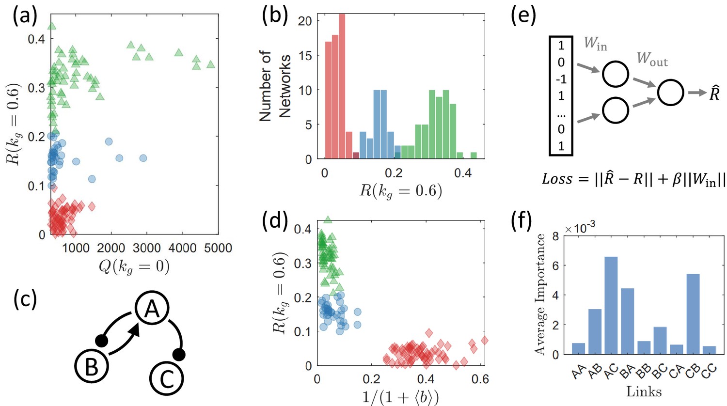
Strong correlation between circuit robustness against growth feedback and circuit topology.

There are three groups of circuits, each displaying strong topological similarities within, exhibit distinct levels of robustness against growth feedback as measured by the characterizing quantity $R$ . (a) Robustness measure $R (k_{g} = 0.6)$ versus $Q (k_{g} = 0)$ for all 425 network topologies. Circuits are color/shape-coded into three groups (green triangles, blue circles, and red diamonds) based on the rules defined in the text. The three groups of topologies display distinct levels of $R (k_{g} = 0.6)$ values, signifying a strong correlation between circuit robustness and topology. Only circuits with $Q (k_{g} = 0) > 300$ are shown to reduce fluctuations arising from random parameter sampling. What is demonstrated is the case of an intermediate level of growth feedback with $k_{g} = 0.6$ (a different value of $k_{g}$ has no significant effect on the results – see Figure 7). The topologies associated with the green triangles have a high level of robustness, which can be regarded as an optimal group and is more prevalent than the optimal group identified in Figure 5. (b) Histogram of $R (k_{g} = 0.6)$ the same color legends as in (a). Three distinct peaks emerge, each associated with a group of circuit topologies. (c) The shared network motif among all networks in the green group, which is highly correlated with the optimal minimal network shown in Figure 5b, but without the link B $\to$ B, which is necessary for the negative feedback loop (NFBL) family of networks to have adaptation (Shi et al., 2017). (d) Effects of burden $b$ for the three groups of networks, where the abscissa is the effective term of burden in the formula of growth rate Equation 12. The circuits in the red group have larger values of $1 / (1 + ⟨ b ⟩)$ , suggesting that a heavier burden yields a stronger effect of the growth feedback for the red group. (e) A multilayer perceptron (MLP) for identifying the crucial connections that determine the robustness of the circuits. The circuit topology serves as the input, where 1, 0, and –1 represent activation, null, and inhibition links, respectively. The output is a predicted robustness measure, denoted as $\hat{R}$ . To encourage the neural network to select as few links as possible for predicting $\hat{R}$ , a l–1 regularization term, $β | | W_{in} | |$ , is incorporated into the loss function alongside the fidelity error $| | \hat{R} - R | |$ . As a result, the feed-forward process eliminates information about the links that have little impact on circuit robustness since the corresponding $W_{in}$ entries automatically optimize to values close to zero. (f) Results from an ensemble of 50 MLPs, each trained with distinct initial values. Shown is the average importance of each of the nine links, which is determined by the weights in $W_{in}$ – see Appendix 8. The top four links with the highest importance correspond to the four links used to classify the three peaks in panel (b).

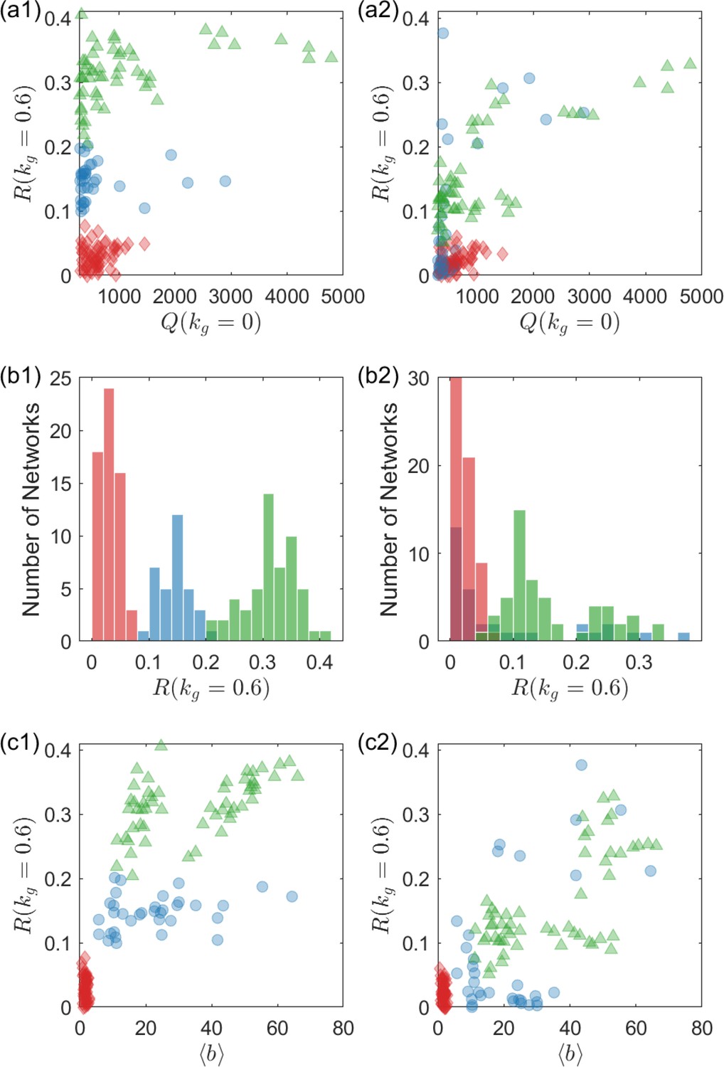
Figure 7

Download asset Open asset

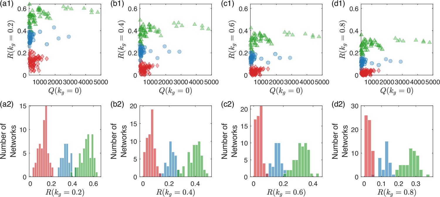
Robustness of the circuit division into three groups subject to different levels of growth feedback.

From the left to the right, the four columns are for (a1, a2) $k_{g} = 0.2$ , (b1, b2) $k_{g} = 0.4$ , (c1, c2) $k_{g} = 0.6$ , and (d1, d2) $k_{g} = 0.8$ , respectively. The legends are the same as in Figure 6a, b. For different levels of growth feedback, the distribution of the robustness measure exhibits three distinct peaks that occur at approximately the same locations on the $R$ axis. The implication is that the division of the circuit topologies into three groups in terms of the robustness measure can be revealed by examining the circuit functions at a single value of the growth-feedback strength.

Figure 8

Download asset Open asset

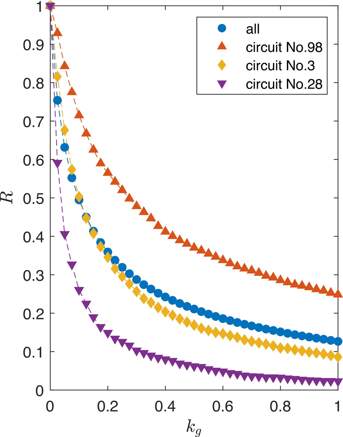
Scaling law governing the circuit robustness measure $R (k_{g})$ .

The blue curve is the average result of all the 425 network topologies. The other three curves represent circuits with different robustness levels: high (Circuit No. 98), moderate (Circuit No. 3), and low (Circuit No. 28) values of $R$ , to demonstrate that this scaling behavior is generic. Each of these three circuit topologies is selected from one of the three groups illustrated in Figures 6 and 7, and they have the highest $Q (k_{g} = 0)$ value within their respective groups.

Appendix 1—figure 1

Download asset Open asset

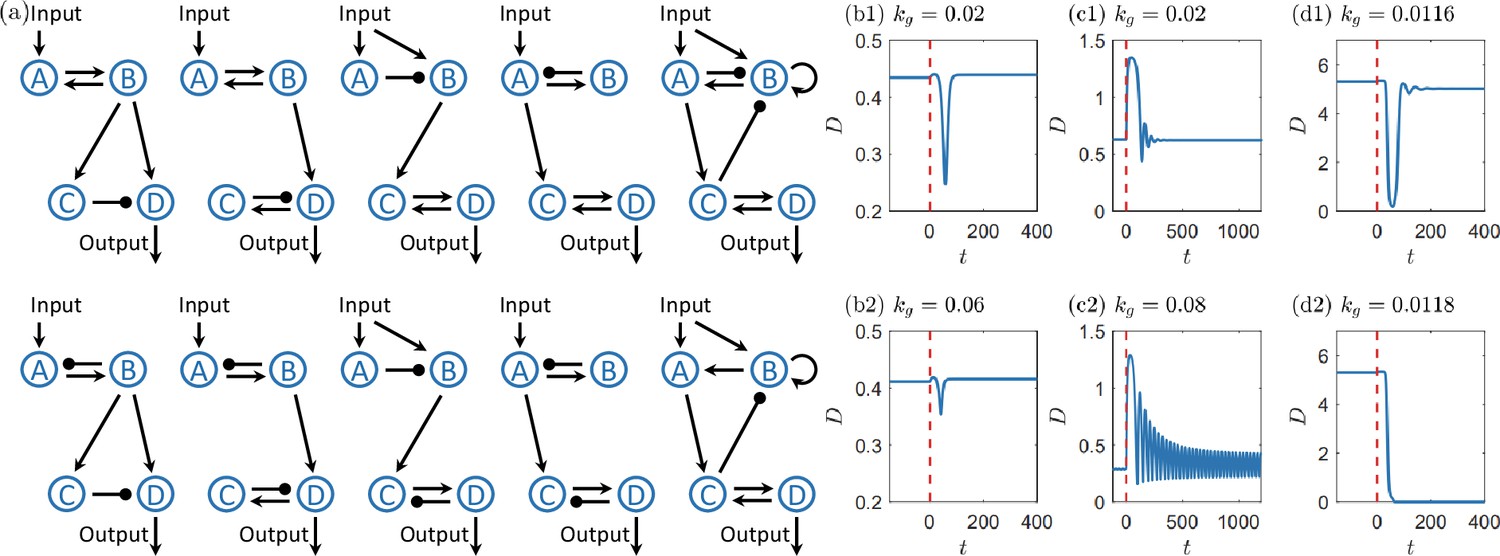
Functional failures in four-gene circuits under growth feedback.

(a) Ten representative four-gene circuits. The eight circuits in the first four columns are from Qiao et al., 2019, and the two circuits in the fifth column are selected due to the oscillation-related motifs in their topologies and the relatively high $Q (k_{g} = 0)$ values when reduced to three-gene circuits. (b–d) Examples of the three major categories of growth-feedback-induced functional failures in the four-gene circuits, where the upper panels display the circuit outputs with smaller $k_{g}$ values for which the circuits remain functional and the lower panels showcase the circuit outputs with larger $k_{g}$ values for which the circuits lose their functionality. The vertical red dashed line marks the time when the input is switched to another state. The three failure categories are identical to these in the three-gene circuits in the main text: (b1, b2) continuous trajectory deformation causing the system to cross thresholds associated with the sensitivity criterion, (c1, c2) growth-strengthened oscillations, and (d1, d2) growth-induced switching in bistability. The change in $k_{g}$ between panels (d1) and (d2) is small so as to show the abrupt change in the response at a critical point.

Appendix 2—figure 1

Download asset Open asset

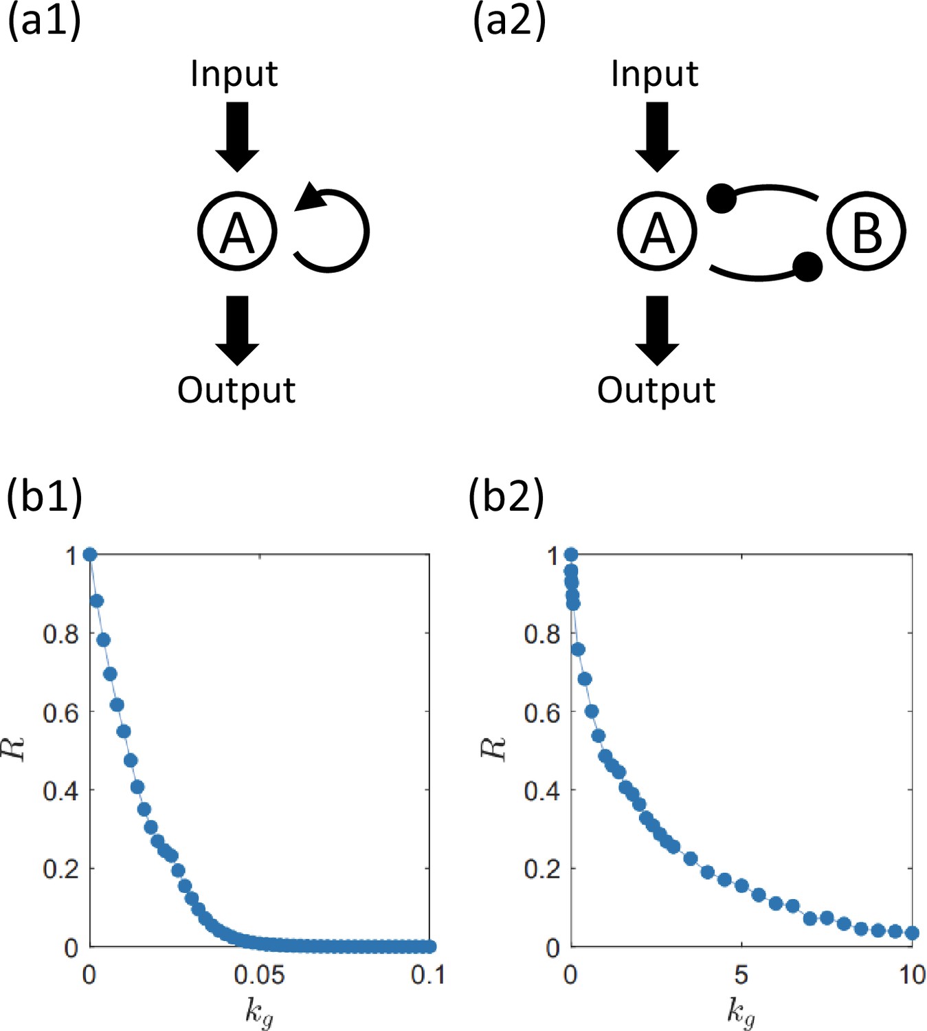
Scaling law of robustness measure for the single-gene self-activation circuit and the two-gene toggle switch circuit.

(a1, b1) The topology of the self-activation circuit and the decay of the robustness measure with the growth-feedback strength. (a2, b2) Same legends as (a1, b1), respectively, for the toggle switch circuit. Note the drastic difference in the range of $k_{g}$ values in (b1) and (b2) where $R$ approaches zero much more quickly in the former than in the latter, indicating the nearly immediate loss of functions of the single-gene circuit even under weak growth feedback.

Appendix 3—figure 1

Download asset Open asset

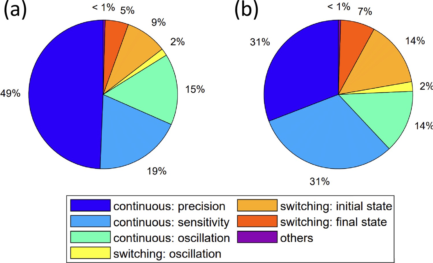
Circuit performance for zero burden.

Shown is a comparison of the distributions of circuit failure scenarios under growth feedback for (a) $J = 1$ as in the main text and (b) $J \to \infty$ (zero burden). In both cases, there are six categories in spite of some quantitative differences in their probabilities, implying that, as the burden is reduced to zero from a finite value continuously, the failure scenarios are qualitatively the same. Notable is the fraction of circuits suffering type-I failures (violation of the precision criterion), which has a relatively large reduction for $J \to \infty$ , a result that is consistent with the semi-quantitative analysis in Appendix 5.

Appendix 3—figure 2

Download asset Open asset

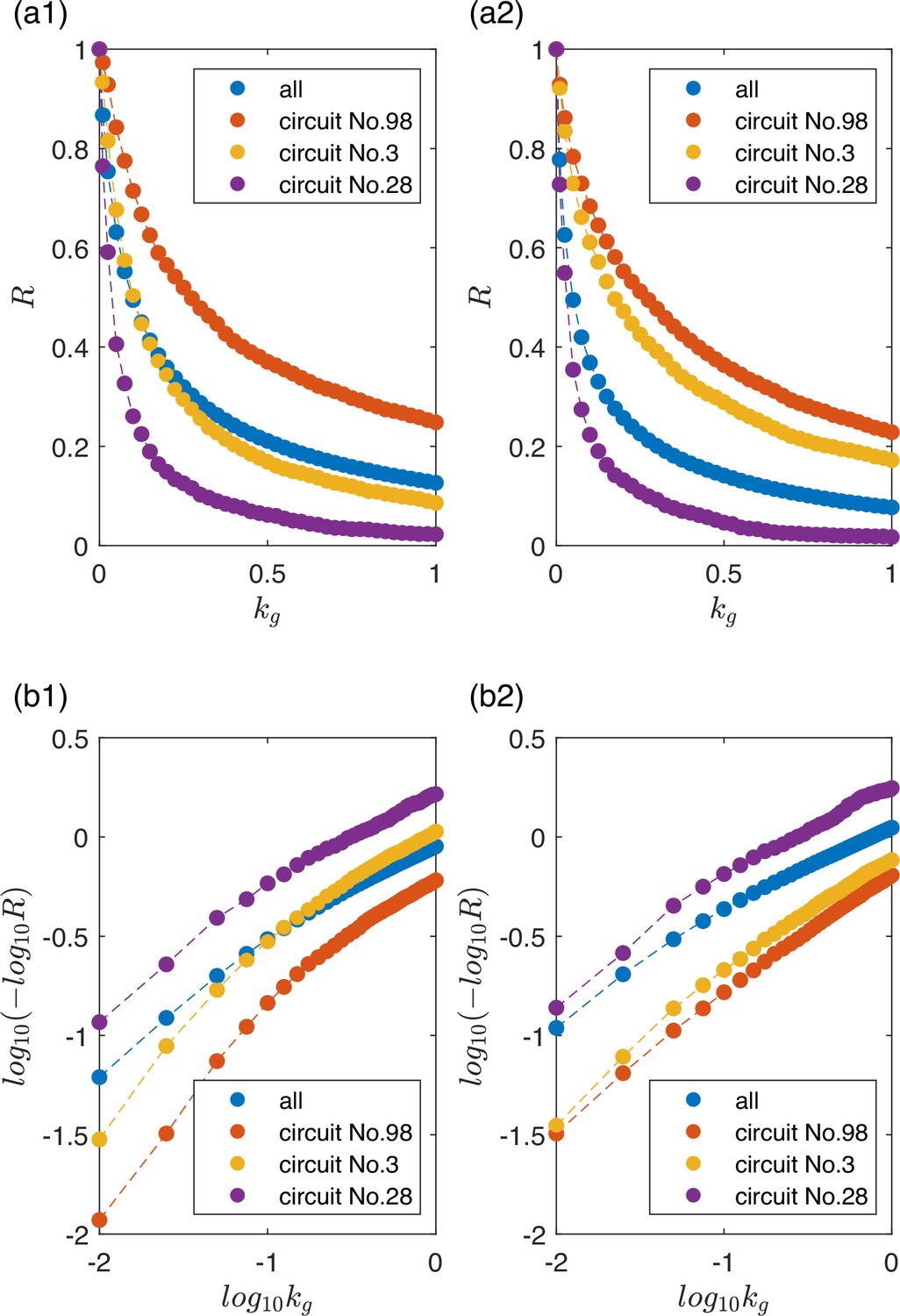
Scaling law of circuit robustness measure for zero burdens.

(a1, b1) Representative scaling relations between $R (k_{g})$ and $k_{g}$ for $J = 1$ as in the main text, plotted on two different scales. (a2, b2) Representative scaling relations for $J \to \infty$ . The curves in (b2) are approximately linear, suggesting the scaling law (1) in the main text. In (b1), the curves are less linear where the added burden leads to more reduction in $R (k_{g})$ in the regime of weak growth feedback.

Appendix 3—figure 3

Download asset Open asset

Dependence of the distribution of the robustness measure $R (k_{g} = 0.6)$ on circuit topology.

(a1) For $J = 1$ (as in the main text), $R (k_{g} = 0.6)$ versus $Q (k_{g} = 0)$ (a quantity that measures the likelihood of a functional circuit) for all 425 network topologies. (b1) Histogram of $R (k_{g} = 0.6)$ for $J = 1$ constructed from all network topologies. (c1) $R (k_{g} = 0.6)$ versus the burden parameter. In (a1–c1), each data point represents a specific network topology. (a2–c2) The same legends as in (a1–c1), respectively, for $J \to \infty$ . Even with the burden removed, the circuit topologies in the red group remain less stable than those in the green group.

Appendix 4—figure 1

Download asset Open asset

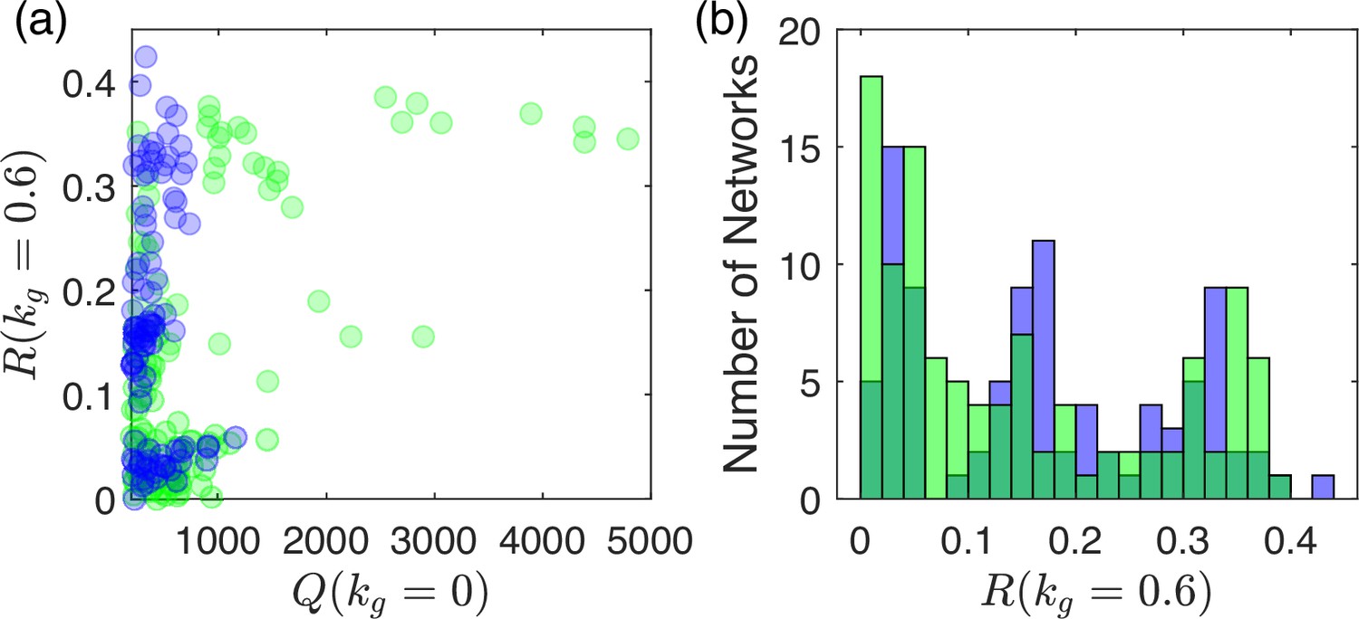
Demonstration of circuit robustness against growth feedback being unrelated to negative feedback loop (NFBL) or feed-forward loop (IFFL) family membership.

The green and blue colors represent the NFBL and IFFL families, respectively. (a) Robustness measure $R (k_{g} = 0.6)$ versus $Q (k_{g} = 0)$ , where each node represents a network topology. Circuits from both families are widely distributed across different levels of $R$ and intermingled. (b) Distributions of $R (k_{g} = 0.6)$ for the two families, which are quite similar.

Appendix 7—figure 1

Download asset Open asset

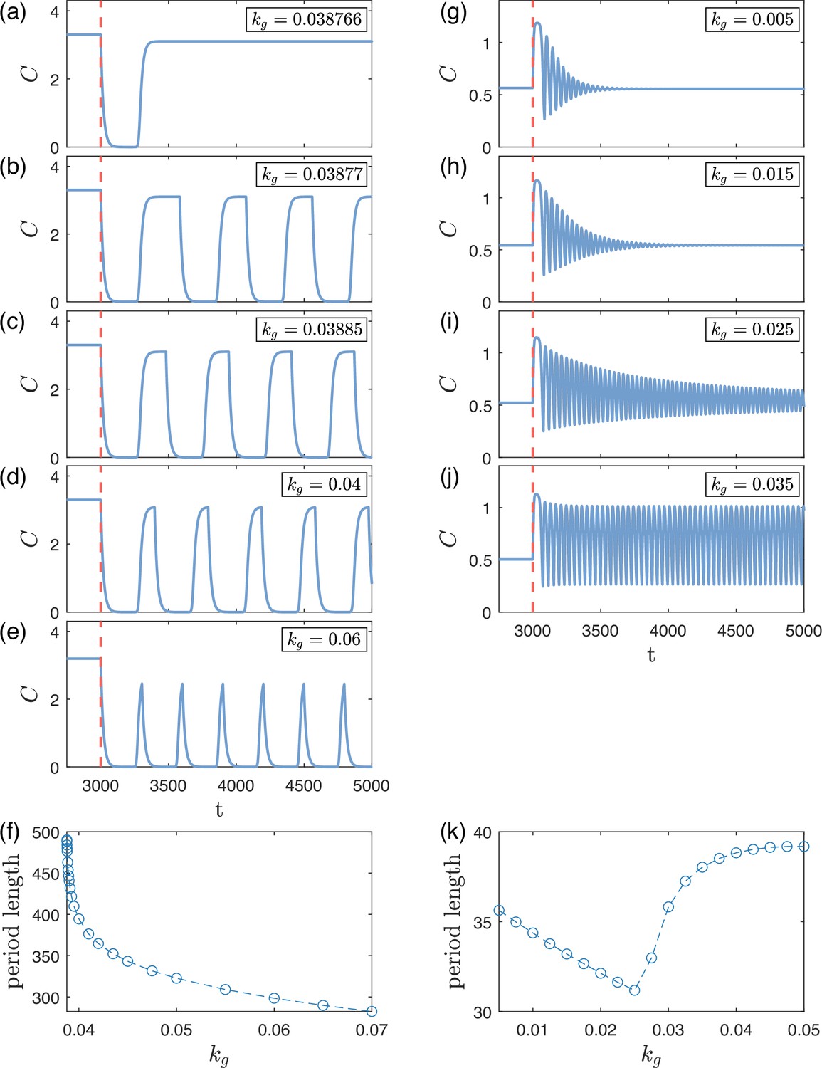
Demonstration of oscillation-related bifurcations.

Here we demonstrate two types of oscillation-related bifurcations: (a–f) infinite-period bifurcation and (g–k) saddle-node bifurcation of cycles. Panels (a–e) show the output signal of a circuit around an infinite-period bifurcation with increasing $k_{g}$ . The circuit fails between panels (a) and (b) due to the emergent oscillation. Panel (f) shows the length of the oscillation period with respect to $k_{g}$ after the critical $k_{g}$ value. There is no persisting oscillation before the critical $k_{g}$ . Panels (g–j) show the output signal of another circuit around a saddle-node bifurcation of cycles with increasing $k_{g}$ . The circuit failed between panels (i) and (j). Panel (k) shows the length of the oscillation period with respect to $k_{g}$ after the critical $k_{g}$ value, where two distinct branches exist on the two sides of the critical $k_{g}$ .

Additional files

MDAR checklist: https://cdn.elifesciences.org/articles/89170/elife-89170-mdarchecklist1-v1.pdf
Download elife-89170-mdarchecklist1-v1.pdf

Download links

A two-part list of links to download the article, or parts of the article, in various formats.

Downloads (link to download the article as PDF)

Article PDF

Open citations (links to open the citations from this article in various online reference manager services)

Mendeley

Cite this article (links to download the citations from this article in formats compatible with various reference manager tools)

Ling-Wei Kong
Wenjia Shi
Xiao-Jun Tian
Ying-Cheng Lai

(2025)

Dynamical mechanisms of growth-feedback effects on adaptive gene circuits

eLife 12:RP89170.

https://doi.org/10.7554/eLife.89170.3

Sign up for email alerts

Privacy notice