Spatial–temporal order–disorder transition in angiogenic NOTCH signaling controls cell fate specification
- Department of Biomedical Engineering, Yale University, United States
- Systems Biology Institute, Yale University, United States
- NSF-Simons Center for Multiscale Cell Fate Research, University of California Irvine, United States
- Department of Mathematics, University of California Irvine, United States
- Center for Theoretical Biological Physics, Rice University, United States
Figures
Figure 1 with 1 supplement
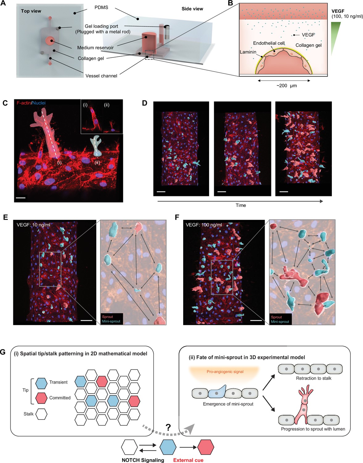
Analysis of temporal and spatial regulation of angiogenic fate specification in a 3D biomimetic experimental setup.
(A) 3D vessel model for inducing angiogenesis in response to a gradient of vascular endothelial growth factor (VEGF). (B) Cross-section of a vessel embedded in collagen type I within the device; VEGF is added to the medium reservoir above the vessel to generate a VEGF gradient. (C) Angiogenesis leads to the formation of new sprout-related structures from the parental vessel that have two distinct morphologies: (i) full-fledged multicellular sprouts containing detectable lumens and (ii) mini-sprouts in the form of single cell extension into the matrix. Scale bars: 20 μm. (D) Temporally resolved observation of dynamic formation of sprouts and mini-sprouts populations during angiogenesis. As depicted in (C), sprouts are pseudo-labeled with red color and mini-sprouts in blue color. Scale bars: 50 μm. Dependence of the spatial distribution of sprouts and mini-sprouts on the VEGF concentration: (E) 10 ng/ml and (F) 100 ng/ml. Scale bars: 50 μm. Images are 3D reconstructions of confocal z-stacks, showing nuclear (Hoechst 33342) and cytoskeleton (Phalloidin). (G) Schematic overview of Tip–Stalk patterning: (i) Spatial Tip–Stalk patterning due to juxtacrine NOTCH signaling that might lead to fixed persistent and transient cell fate specification. (ii) Fates of mini-sprouts in experiments: both retraction (thus conversion from the phenotypically Tip to as Stalk phenotype) and stabilization and growth to a fully defined sprout are observed.
Figure 1—figure supplement 1
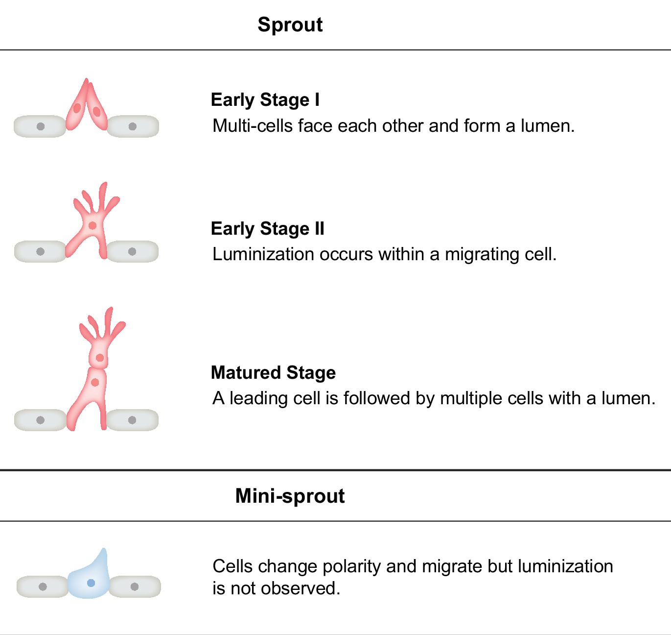
Phenotypic categorization of sprout and mini-sprout.
Figure 2 with 1 supplement
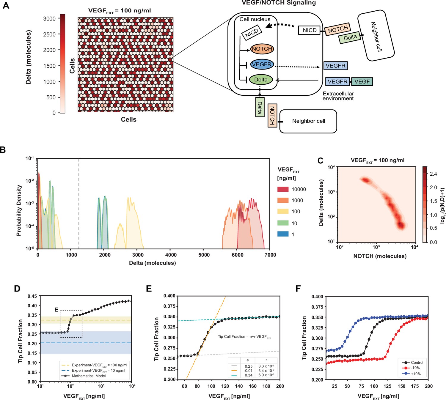
Robust differentiation and order–disorder transition are suggested by mathematical and experimental analyses.
(A) Right: An example of a pattern after full equilibration on a 30 × 30 hexagonal lattice. Color scale highlights the intracellular levels of Delta. Left: The circuit schematic highlights the components of the intracellular NOTCH–vascular endothelial growth factor (VEGF) signaling network. (B) Distribution of intracellular Delta levels in the two-dimensional lattice for increasing levels of external VEGF stimuli. (C) Pseudopotential landscape showing the distribution of intracellular levels of NOTCH and Delta for VEGFEXT = 100 ng/ml. (D) Fraction of Tip cells as a function of external VEGF stimulus (black curve). Blue and yellow lines and shading depict experimental fractions of Tip cells for VEGFEXT = 10 ng/ml and VEGFEXT = 100 ng/ml, respectively. (E) Detail of Tip cell fraction transition zone (corresponding to box in panel D). Legend depicts the coefficients of the linear fits. (F) Shift of the VEGFEXT transition threshold upon variation of the NOTCH–Delta-binding rate constant. For panels B–F, results are averaged over 50 independent simulations starting from randomized initial conditions for each VEGFEXT level (see Methods: Simulation details).
Figure 2—figure supplement 1
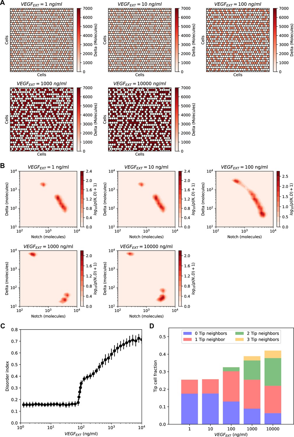
Order–disorder transition in the NOTCH–Delta–vascular endothelial growth factor (VEGF) multicell model.
(A) Steady-state patterns for increasing levels of VEGF signal. Red heatmaps show the levels of Delta in each lattice cell. (B) Pseudopotential landscape of the joint (NOTCH, Delta) intracellular levels for increasing levels of VEGF signal. (C) The disorder index of the pattern as a function of external VEGF signal. The disorder index is defined as the fraction of ‘incorrect’ Tip–Tip contacts in the lattice. (D) Statistics of Tip–Tip contacts as a function of external VEGF signal. For each VEGF input level on the x-axis, the bar height represents the overall fraction of Tip cells in the pattern, while the color-coding classifies Tip cells based on the number of ‘incorrect’ Tip nearest neighbors. For panels (B–D), results are averaged over n = 50 independent simulations starting from randomized initial conditions on a 30 × 30 hexagonal lattice with periodic boundary conditions (see methods for details).
Figure 3
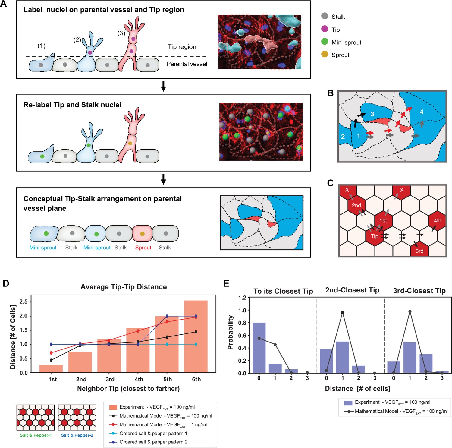
Experimentally measured spatial distribution of Tip cells defined as constituting mini-sprouts and leading sprouts is consistent with the mathematical model predictions.
(A) Analysis pipeline to infer the 2D Tip–Stalk arrangements from 3D experimental images: experimental labeling of the nuclei of sprout/mini-sprout cells (above the plane of the parental vessel) and of the Stalk cells (below the plane of the parental vessel) is used to ‘compress’ the cells in each sprout or mini-sprout into a single Tip cell. Tip–Tip distance is defined as the number of cells measured in ‘cell hops’, that is, the minimal number of intermediate cells between randomly chosen pairs of Tip cells from experiments (B) (the example is identical to the inset at the bottom of (A)) and 2D Tip–Stalk patterns from mathematical modeling (C). Black arrows indicate minimal and valid cell hops between Tips, whereas gray arrows indicate minimal but invalid cell hops (passing through other Tip cells); red arrows indicate the non-minimal cell hops which does not count in the Tip–Tip distance quantification. (D) Tip cell distance distribution from any given Tip cell. Red bars depict experimental measurement for VEGFEXT = 100 ng/ml and black line depicts the model’s prediction for VEGFEXT = 100 ng/ml. For reference, dashed lines indicate the expected Tip–Tip distance distribution of ‘perfect’ salt-and-pepper patterns shown in the inserts. (E) Detailed distance distribution for the closest Tip (left), second closest Tip (middle), and third closest Tip (right).
-
Figure 3—source data 1
Raw data for Tip–Tip distance measurements in Figure 3D, E.
- https://cdn.elifesciences.org/articles/89262/elife-89262-fig3-data1-v2.xlsx
Figure 4
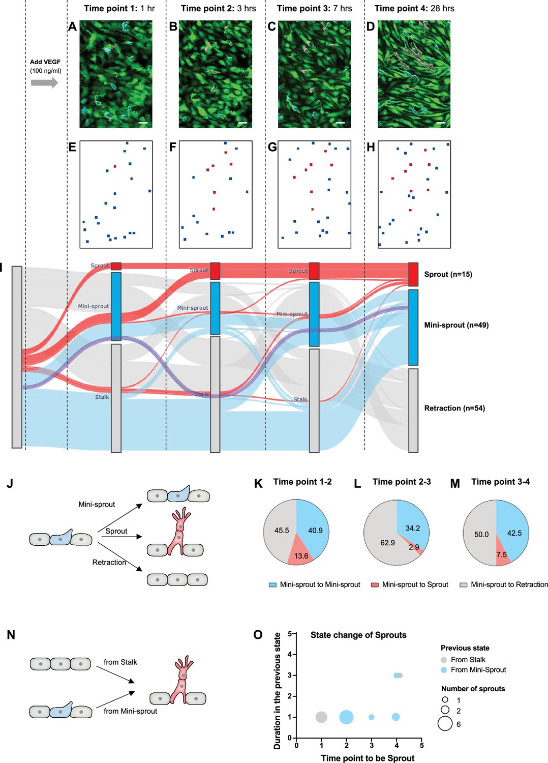
The dynamics of mini-sprout and sprout formation suggest frequent mini-sprout retractions, since only a subset of mini-sprouts becoming fully formed sprouts.
Green fluorescent protein (GFP)-expressing endothelium in the 3D vessel setup captured 1 hr (A), 3 hr (B), 7 hr (C), and 28 hr (D) after 100 ng/ml of vascular endothelial growth factor (VEGF) treatment. Sprouts and mini-sprouts are identified by red and blue surface entities, respectively. Square marks representing the positions of sprouts (red) and mini-sprouts (blue) in the original images at each time point (E–H). (I) Sankey diagram demonstrating the dynamic state change of sprouts with red lines and mini-sprouts with blue lines throughout the time points. And gray lines represent mini-sprouts which ended up being retracted at the last observation, time point 4. A purple line shows an example of the state change from a Stalk (initially non-invading endothelial cell) to mini-sprout, retraction, mini-sprout, and mini-sprout at each time point. Only cells that that became mini-sprout at least once during the experiment are shown. (J) Different types of observed transitions between consecutive time points when starting from the mini-sprout state: maintain the mini-sprout state, become a sprout, or retract to the Stalk state. The ratio of states switched from mini-sprouts in the previous time point 1 (K), time point 2 (L), and time point 3 (M). (N) The two observed pathways to sprout formation between consecutive time points: direct Stalk to sprout or mini-sprout to sprout transition. Once a newly formed vessel becomes a sprout, it is permanently committed. (O) Duration of staying as a mini-sprout or a Stalk in the previous state before being committed to a sprout.
-
Figure 4—source data 1
Raw data tracking the dynamics of mini-sprout and sprout formation in each timeframe for Figure 4I–O.
- https://cdn.elifesciences.org/articles/89262/elife-89262-fig4-data1-v2.xlsx
Figure 5 with 1 supplement
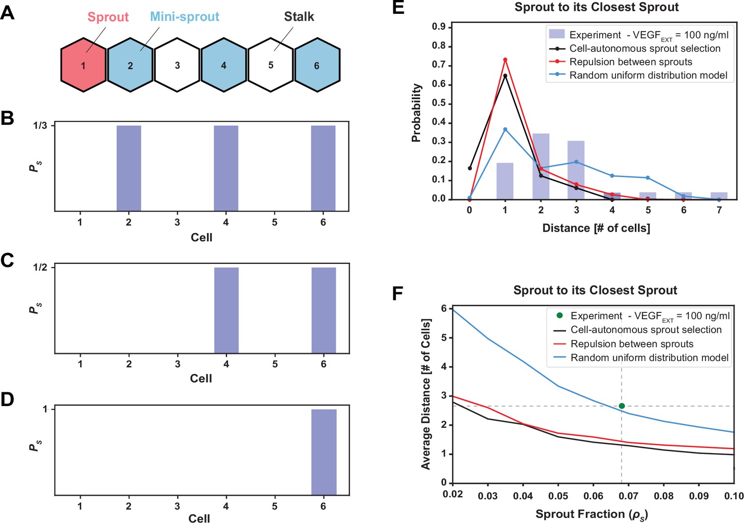
The phenomenological model favoring maximal sprout–sprout distances for a given number of sprouts (random uniform distribution) is most consistent with the experimental observations.
(A) An example of one-dimenstional Tip cell distribution, including a sprout and mini-sprouts, and Stalks pattern. (B) Sprout selection probability (PS) for the cell-autonomous model if a new sprout was added to the pattern of (A). Stalk cells cannot become sprouts, and existing mini-sprouts share the same selection probability. (C) Sprout selection probability (PS) for the sprout repulsion model. The leftmost mini-sprout cannot be selected because it is already in contact with an existing sprout, while the remaining two mini-sprouts share the same selection probability. (D) Sprout selection probability (PS) for the random uniform distribution model. The rightmost mini-sprout maximizes the distance to the existing sprout and is therefore the only viable selection. (E) Sprout distance distribution to its closest sprout neighbor. Blue bars indicate experimental results for VEGFEXT = 100 ng/ml while black, red, and blue lines depict the three different models of sprout selection (cell-autonomous, repulsion between sprouts, and random uniform distribution, respectively). (F) Average distance between a sprout and its closest sprout neighbor in the model as a function of sprout cell fraction in the lattice for the three proposed models of sprout selection. The green dot highlights the experimental sprout fraction and distance at VEGFEXT = 100 ng/ml.
Figure 5—figure supplement 1

Phenomenological models of Sprout selection.
(A) Detailed distribution of Sprout distance to its closest Tip neighbor. Solid blue bars depict experimental measurements for the vascular endothelial growth factor (VEGF) =100 ng/ml experiment, while black, red, and green lines depict the predicted distance distributions for the cell-autonomous, repulsion, and random uniform Sprout selection models. (B–D) Distribution of Sprout distance to its closest Sprout neighbor predicted by the model. Different curves indicate the Sprout distance distribution for models with increasing Sprout cell density ranging from 2% to 10% (the experimental sprout density at VEGF =100 ng/ml is ). Panels B–D depict predictions for the cell-autonomous, repulsion between sprouts, and random uniform sprout selection models, respectively. In all panels, the VEGF level is fixed to VEGF =100 ng/ml to match the experimental model.
Figure 6
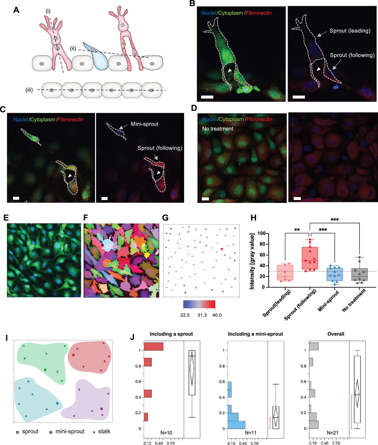
Fibronectin distribution on parental and newly formed vessels reveals preferred distribution at the bases of sprouts.
(A) A schematic describing cross-sectional planes for subsequent confocal images: (i) for (B), (ii) for (C), and (iii) for (D). (B) Localization of fibronectin expression to a following cell than in a leading cell in a sprout. (C) Higher fibronectin expression in a sprout (a ‘following’ cell at the base of the sprout) than at a mini-sprout. (D) Intrinsic heterogeneity of fibronectin expression on quiescent endothelium displaying no mini-sprout or sprout formation. Images are 3D reconstructions of confocal z-stacks. Scale bars: 15 μm. Cells on the parental vessel were identified by GFP expression in the cytoplasm (E), then segmented (F). (G) Fibronectin intensity of each cell on the parental vessel is marked as a dot at the corresponding x and y positions of the cell centroids. Fibronectin intensities for sprouts (following cells) or mini-sprouts are indicated as squares. (H) Fibronectin intensity of leading cells and following cells of sprouts, mini-sprouts, and quiescent cells. Data are presented by box and whiskers with all individual points representing each cell (Nsprout(leading): 7; Nsprout(following): 11; NMini-sprout: 11; NNo treatment: 10). One-way ANOVA analysis was performed followed by Tukey’s multiple comparisons test (*p < 0.05, **p < 0.01, ***p < 0.001, ****p < 0.0001). (I) Cellular layer was segmented into groups containing seven neighboring cells to assess the local environment for each group. (J) Distributions of the ratio of cells having fibronectin levels higher than a threshold, the minimum value of sprout in (H), in a group of seven neighboring cells defined in (I), which included either a sprout or a mini-sprout. The overall distribution covers both regions.
-
Figure 6—source data 1
Raw fibronectin intensity data for Figure 6H, J.
- https://cdn.elifesciences.org/articles/89262/elife-89262-fig6-data1-v2.xlsx
Tables
Key resources table
| Reagent type (species) or resource | Designation | Source or reference | Identifiers | Additional information |
|---|---|---|---|---|
| Antibody | Recombinant Anti-Fibronectin antibody (Rabbit monoclonal) | abcam | ab268020 | IF (1:50) |
| Antibody | Goat anti-Rabbit IgG (H+L) Highly Cross-Adsorbed Secondary Antibody, Alexa Fluor Plus 594 (Goat polyclonal) | Invitrogen | A32740 | IF (1:100) |
| Peptide, recombinant protein | Animal-Free Recombinant Human FGF-basic (bFGF) | PeproTech | AF10018B | |
| Peptide, recombinant protein | VEGF Recombinant Human Protein | Life Technologies | PHC9394 | |
| Chemical compound, drug | Sphingosine-1-phosphate | Sigma-Aldrich | S9666 | |
| Chemical compound, drug | Phorbol myristate acetate | Sigma-Aldrich | P1585 | |
| Biological sample (Homo sapiens) | Primary human brain microvascular endothelial cells transfected with GFP-expressing lentivirial particles. | Angio-Proteomie | cAP-0002GFP | Isolated from normal human brain tissue |
| Software, algorithm | IMARIS 9.8.0 | Bitplane | https://imaris.oxinst.com | |
| Software, algorithm | PRISM 9.0.0 | GraphPad | https://www.graphpad.com/features | |
| Software, algorithm | Jupyter Notebook 6.1.6 | Project Jupyter | https://jupyter.org/install | |
| Software, algorithm | Python 3.12.1 | Python Software Foundation | https://www.python.org | |
| Other | Hoechst 33342 | Thermo Fisher | H3570 | IF (5 µg/ml) |
Table 1
Parameter values for simulation.
| Parameter type | Parameter | Value | Units |
|---|---|---|---|
| Production | , , , | 1200, 1000, 800, 1000 | Molecule/hr |
| Degradation | , | 0.1, 0.5 | 1/hr |
| Binding | , | 2.5 × 10⁻⁵, 5 × 10⁻⁴ | 1/(molecule hr) |
| Hill threshold | , | 200, 80* | Molecules |
| Fold-change | , , , , | 2, 0, 0, 2, 2 | Dimensionless |
| Hill coefficient | , , , , | 2, 2, 2, 5, 2 | Dimensionless |
-
*
Rescaled from previous model to match experimental observation.
Additional files
-
MDAR checklist
- https://cdn.elifesciences.org/articles/89262/elife-89262-mdarchecklist1-v2.docx
-
Source code 1
Source code for mathematical modeling.
This includes all codes used in the mathematical modeling for Figure 2, Figure 2—figure supplement 1, Figure 3, Figure 5, and Figure 5—figure supplement 1.
- https://cdn.elifesciences.org/articles/89262/elife-89262-code1-v2.zip
Download links
A two-part list of links to download the article, or parts of the article, in various formats.
Downloads (link to download the article as PDF)
Open citations (links to open the citations from this article in various online reference manager services)
Cite this article (links to download the citations from this article in formats compatible with various reference manager tools)
Spatial–temporal order–disorder transition in angiogenic NOTCH signaling controls cell fate specification
eLife 12:RP89262.
https://doi.org/10.7554/eLife.89262.3


