Task-anchored grid cell firing is selectively associated with successful path integration-dependent behaviour
Figures
Models for grid representation and experiment design.
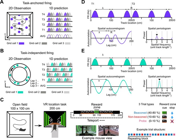
(A–B) Predicted task-anchored (A) and task-independent (B) firing of grid cells in a 1D environment (right) given firing patterns of grid cells previously observed in square (A) and circular (B) 2D arenas (left). T1-T4 indicate consecutive trials in the 1D environment, AVG indicates expected average across many trials. (C) Neurons were recorded in an open arena and then in a location memory task. Trials were configured with a reward for stopping in a visually cued zone (beaconed), or a reward for stopping in the same zone but with the cue absent (non-beaconed), or without the visual cue or the reward (probe). Trial percentages indicate the proportion of trial types experienced in a single session; in any given session this proportion was fixed and trials were interleaved in a fixed repeating pattern (see Materials and methods). (D) In the task-anchored coding scheme, a grid cell fires with field spacing λ and resets its firing every trial by anchoring its fields to the same track location, with a realignment lag R observed in the spatial autocorrelogram. Fields locations remain constant on each trial and thus peaks in the periodogram occur at integer spatial frequencies relative to the track repetition (see Figure 1—figure supplement 3). (E) In a task-independent coding scheme, a grid cell fires with field spacing λ and continues to fire at regular intervals without anchoring to the track. Unless field spacing and the track length are integer divisible, the location of fields varies across trials, and thus the peak of the periodogram is not constrained to an integer spatial frequency (see Figure 1—figure supplement 3).

Procedure for extracting a session-level periodogram from a set of spike timestamps.
A single cell’s spikes were binned in space (1 cm bin size), divided by the time spent in each bin then smoothed using a Gaussian kernel (SD = 2 cm). Least squares spectral analysis (LSSA) was computed on a signal equivalent to three track lengths using the Lomb-Scargle implementation in the Astropy Python module (Δx=distance elapsed in trials, Δy=firing rate)(Price-Whelan et al., 2022). The signal was advanced 10 cm and repeated for the whole session. All individual periodograms generated were then used to generate the average periodogram.

Procedure for estimating a false alarm threshold for a given cell.
To generate shuffled datasets a cell’s spikes were first binned in space (1 cm bin size), divided by the time spent in each bin then smoothed using a Gaussian kernel (SD = 4 cm). Firing fields were detected and the original field bins reallocated to random locations on a new unsmoothed rate map. Bins not attributed to a field were allocated to the remaining gaps in the new map. The unsmoothed shuffled rate map was then smoothed with a Gaussian kernel (SD = 2 cm). An average periodogram was calculated and peak power detected. This was repeated 1000 times. The false alarm threshold was set equal to the 99th percentile of the peak power of periodograms generated from the shuffled dataset.
Identification of task-anchored and task-independent periodic firing.
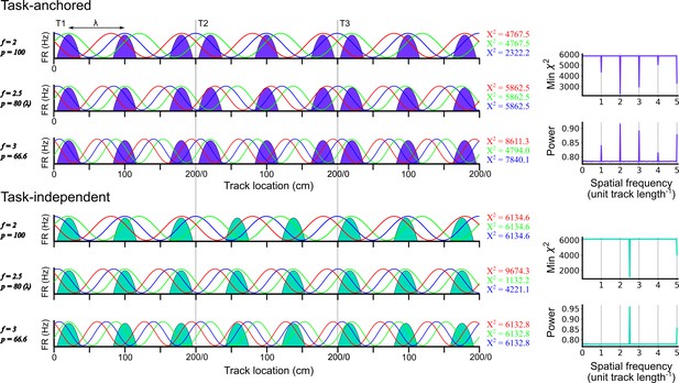
Examples of least squares spectral analysis (LSSA) used to estimate the sinusoidal components that best describe the firing rate profile of a task-anchored grid code (upper) and a task-independent code (lower). In each plot the schematised firing fields (solid colours) are shown as a function of track position. Each row shows examples of different sinusoidal components (f=frequency, p=period) at different phases. LSSA minimises the chi-squared error by searching over all phases (three example phases are shown in red, green, and blue per row) and amplitudes (amplitude is ignored here for simplicity) for each spatial frequency. For task-anchored grid representations, the chi-squared error (min χ2) is minimal at positive-integer spatial frequencies that correspond to sinusoidal waves with periods that are integer divisible by the track length. For task-independent grid representations the chi-squared error is minimal at a spatial frequency that corresponds to the underlying periodic firing rate profile. The standard normalised periodogram is created by normalising the chi-squared errors of the periodic model around a non-varying reference model. The resulting power is a dimensionless quantity that lies within the range 0–1.
Expected spatial periodicity for different functional cell types.
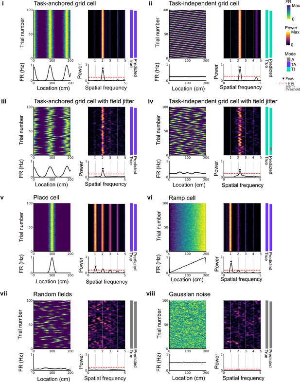
Plots show simulations of track firing for (i) a task-anchored grid cell, (ii) a task-independent grid cell, (iii) a task-anchored grid cell with field jitter, (iv) a task-independent grid cell with field jitter, (v) a place cell, (vi) a ramp-like cell, (vii) a cell with randomly positioned fields, and (viii) a cell with Gaussian noise-like activity. Each group of panels shows firing rate heat map by trial (upper left) and corresponding average firing rate (lower left), rolling periodogram (upper centre) and corresponding average periodogram (lower centre), the true and predicted trial classification (upper right). The predicted trial classification is established using analyses described in Figure 1—figure supplements 1–3.

Validation of accuracy and bias for classification of task-anchored and task-independent modes.
500 task-anchored grid cells and 500 task-independent grid cells with grid spacings uniformly distributed between 40 and 400 cm were simulated to identify the optimal threshold to classify based on spatial frequency. Simulations were repeated using different spike rate probabilities and different field jitters (defined by the standard deviation of the field locations from their preassigned locations). Roughly, Pmax(spike) values of 0.01, 0.1, and 1 covered average firing rates on the order of magnitudes of 10–1, 100, 101 Hz respectively whereas jitter SD values of 0, 10, 20, and 30 cm covered progressively greater deviations from perfect periodic firing. Classifications were made on each set of simulations in the same way as for analysis of experimental data (see Figure 1—figure supplements 1–4). Prediction accuracy (left) and bias (right) are shown as a function of the spatial frequency from the nearest positive-integer used as a threshold to distinguish task-anchored and task-independent modes. Chance level accuracy is denoted with a red dashed line.
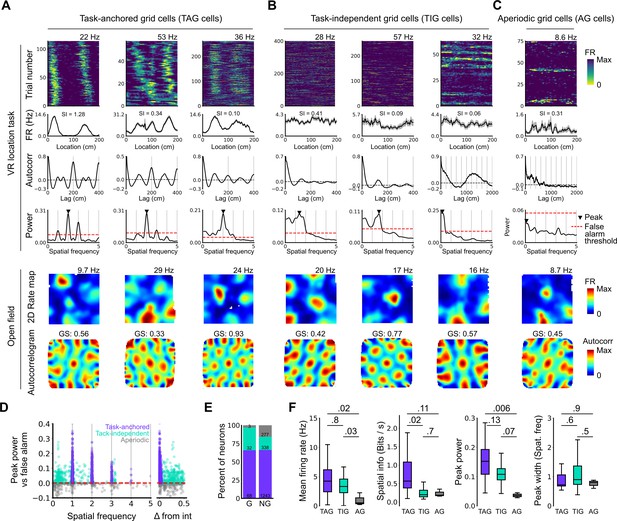
Grid cells operate in task-anchored or task-independent firing modes.
(A–C) Examples of grid cells with activity during the location memory task classified as task-anchored (A), task-independent (B), or aperiodic (C) at the session level. Examples are ordered in their respective groups by their spatial information on the track. From top to bottom plots show: heap map of firing rate as a function of track position, spatial autocorrelation of the track firing rate, periodogram of the track firing, open field firing rate map, and open field spatial autocorrelogram. The red line indicates the false alarm threshold estimated from shuffled data and significant peaks are labelled with a triangle. X-axis scales are adjusted on the virtual reality spatial autocorrelation to better illustrate the long-range periodic signal. (D) Peak power as a function of the spatial frequency at which the peak occurs for all recorded cells. The red dashed line indicates the false alarm threshold generated from shuffled data. (E) Percentage of grid (G) and non-grid (NG) cells classified to task-anchored, task-independent, and aperiodic groups. (F) Comparison between task-anchored (TAG), task-independent (TIG), and aperiodic (AG) grid cells of mean firing rate (ANOVA: DF=2, p=0.006, Χ2=10.215; pairwise comparisons: TAG vs TIG, DF=4.12, p=0.8, T=0.562; TAG vs AG, DF=42.07, p=0.02, T=2.906; TIG vs AG, DF=67.29, p=0.03, T=2.588), spatial information scores (ANOVA: DF=2, p=0.008, Χ2=9.54; pairwise comparisons: TAG vs TIG, DF=73.6, p=0.02, T=2.815; TAG vs AG, DF=95.5, p=0.11, T=2.036; TIG vs AG, DF=96.6, p=0.7, T=0.783), peak power (ANOVA: DF=2, p=0.001, Χ2=13.792; pairwise comparisons: TAG vs TIG, DF=19.0, p=0.13, T=2.033; TA vs A, p=0.006, T=3.239, DF=54.9; TI vs A, p=0.07, T=2.274, DF=80.4), and peak width (ANOVA: DF=2, p=0.15, Χ2=3.7963; pairwise comparisons: TAG vs TIG, p=0.61, T=–1.029, DF=3.27; TA vs A, p=0.88, T=0.472, DF=45.76; TI vs A, p=0.55, T=1.053, DF=71.22).
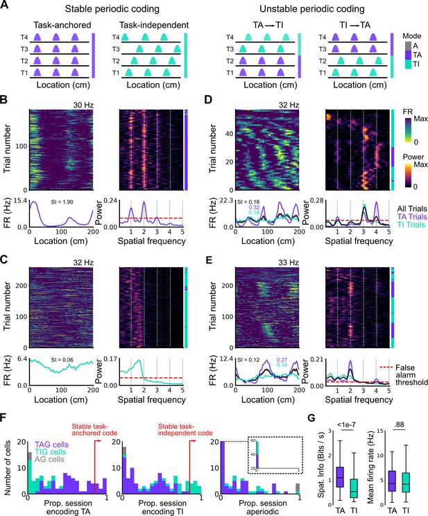
Coding schemes switch within behavioural sessions.
(A) In a ‘stable coding’ scenario grid cells remain either task-anchored or task-independent throughout the recording session (left), whereas with ‘unstable coding’ the grid activity switches between task-anchored and task-independent modes (right). (B–E) Example trial-by-trial firing rate heat maps (upper left), corresponding rolling periodogram heat maps (upper right), mean rate maps (lower left), and mean periodograms (lower right) for neurons exhibiting stable task-anchored coding (B), stable task-independent coding (C), and unstable coding in which representations switch between task-anchored and task-independent (D–E). (F) Distribution across all recorded grid cells of task-anchored trials (left), task-independent trials (centre), and aperiodic trials (right). Session-level task-anchored grid (TAG), task-independent grid (TIG), and aperiodic grid (AG) cell classifications are differently coloured. (G) Spatial information was higher for trials when grid cells were task-anchored compared to when they were task-independent (left) (ANOVA: p<1e-7, Χ2=30.98, DF=1), whereas the average firing rate was similar between task-anchored and task-independent trials (right) (ANOVA: p=0.88, Χ2=0.022, DF=1).

Procedure for classifying periodicity on a rolling basis.
Periodograms were generated as in Figure 1—figure supplement 1. Sliding windows containing 200 consecutive periodograms were then extracted and averaged. A classification was made on the averaged periodogram using the peak power, spatial frequency, and an adjusted false alarm threshold (see Materials and methods). The classification and midpoint location of the window were stored and the procedure repeated for the full session. Windows were assigned to trials based on the location of their middle points and then the classification occurring most often was assigned to that trial.
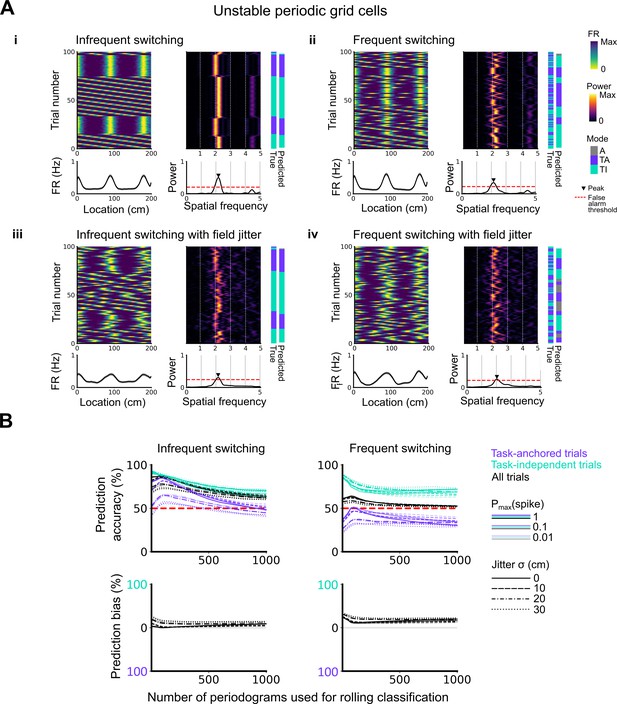
Evaluation of classification accuracy and bias as a function of the number of periodograms used for rolling classification.
(A) Examples of the activity of simulated grid cells that switch between task-anchored and task-independent encoding modes of operation, either infrequently (i, iii) or relatively frequently (ii, iv), and with (iii, iv) and without (i, ii) jitter. Each example shows the firing rate heat map by trials (upper left), the average firing rate map (lower left), the rolling periodogram (upper right), the average periodogram (lower right), and the classification labels (true and predicted; far right). (B) To assess classification accuracy under different rolling windows, we calculated the prediction accuracy and bias (see Materials and methods). Chance level is denoted with a red dashed line. Plots on the left show the prediction accuracy (top) and the prediction bias (bottom) when grid cells alternate between task-anchored and task-independent firing fields in blocks of trials (as in i, iii above), whereas the right plots show the same information for a higher switching frequency (as in ii, iv above).
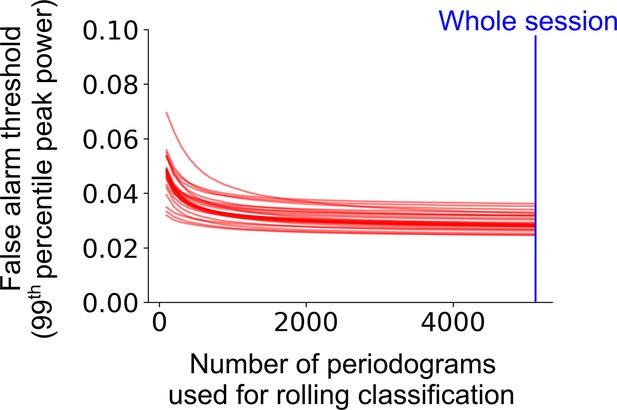
Classification accuracy and bias on the level of trial as a function of rolling window size.
The false alarm threshold was defined by the 99th percentile of the distribution of the peak power of the average periodogram for 1000 shuffled instances of a cell’s firing rate profile across the full experimental session. The false alarm threshold decreases asymptotically as the number of periodograms used for the rolling window classification is increased. Each red line represents a single cell within a representative session. The blue line represents the maximum number of periodograms in this session.
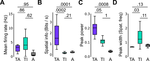
Spatial firing properties of stable task-anchored and task-independent grid cells.
This is a repeat of the analysis shown in Figure 2F, but categorising cells according to the proportion of trials on which their firing is a given mode. Thus, whereas in Figure 2 task-anchored, task-independent, and periodic firing classifications are assigned on the basis of average periodograms across the behavioural session, here we group cells according to whether they show stable (>85% of trials) task-anchored, task-independent, or periodic firing. Conclusions from this analysis are similar to those of Figure 2F. (A) Comparison of mean firing rate (ANOVA: p=0.49, Χ2=1.42, DF=2; pairwise comparisons: TA vs TI, p=0.86, T=–0.532, DF=21.4; TA vs A, p=0.95, T=–0.292, DF=96.7; TI vs A, p=0.62, T=–0.937, DF=23.1). (B) Comparison of spatial information scores (ANOVA: p<1e-4, Χ2=21.47, DF=2; pairwise comparisons: TA vs TI, p=0.0002, T=4.229, DF=89.9; TA vs A, p=0.0001, T=–4.412, DF=94.2; TI vs A, p=0.21, T=1.703, DF=85.2). (C) Comparison of peak power (ANOVA: p=0.0007, Χ2=14.42, DF=2; pairwise comparisons: TA vs TI, p=0.05, T=2.383, DF=88.4; TA vs A, p=0.0008, T=–3.781, DF=98.9; TI vs A, p=0.996, T=–0.080, DF=86.5). (D) Comparison of peak width (ANOVA: p=0.002, Χ2=12.78, DF=2; pairwise comparisons: TA vs TI, p=0.03, T=–2.840, DF=16.2; TA vs A, p=0.13, T=1.949, DF=95.3; TI vs A, p=0.11, T=–2.162, DF=16.0).
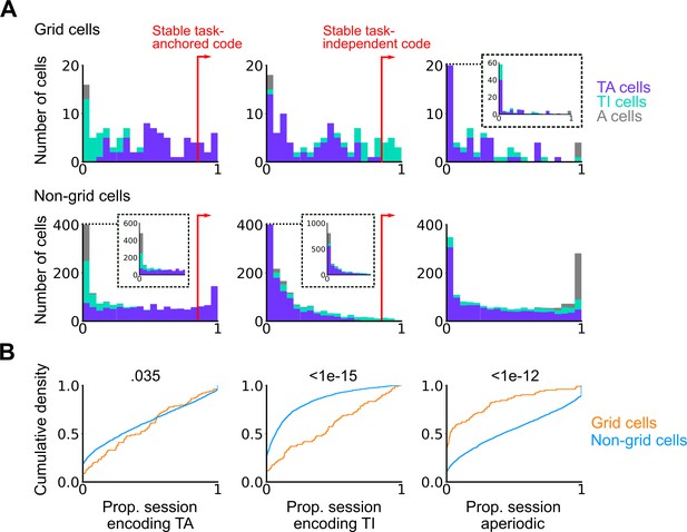
Grid cells exhibit task-independent periodic codes more frequently than non-grid cells.
Extension of Figure 3F. (A) Distribution of all recorded grid cells (top) and non-grid cells (bottom) encoding task-anchored (left), task-independent (centre), and aperiodic (right) epochs within a session. Session-level cell classifications are represented by the colour of the corresponding coding group. (B) Cumulative density for grid and non-grid cells encoding task-anchored, task-independent, and aperiodic epochs within a recording session (task-anchored: p=0.035, KS=0.14; task-independent: p<1e-15, KS=0.42; aperiodic: p<1e-12, KS=0.38, Ngrid cells = 103, Nnon-grid cells = 1778, Kolmogorov-Smirnov test).
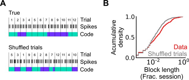
Assessment of the length of periodic coding blocks.
(A) We compared the length of coding blocks - sequences of trials in which grid cells operate in the same mode - in the observed data with the length in datasets shuffled at the level of trials. To generate shuffled data spike locations were reallocated to a new position in the firing profile by randomly shuffling the trials (see Materials and methods). The rolling classification was then recomputed and length of coding blocks measured. (B) Cumulative histogram of block lengths for the observed grid cell population (red) and the same grid cell population with the trial order shuffled and blocks recalculated (grey) (p=0.0003; KS=0.066; Nblocks(data)=1765 Nblocks(shuffled)=2359; Kolmogorov-Smirnov test).
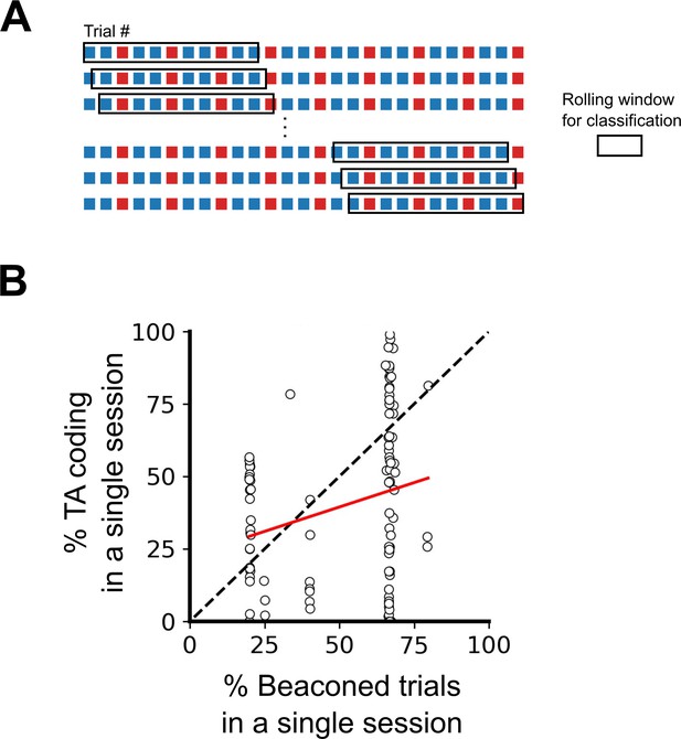
Differences in order and ratio of trial types do not explain the variability in task-anchoring.
(A) Example trial structure with repeating beaconed and non-beaconed trials in a ratio of two beaconed trials to one non-beaconed trial. The rolling window over which the rolling classification of periodicity is calculated is larger than the repeating trial block. Therefore, attribution of a periodic classification to a single trial cannot be explained by the trial type or order. (B) The percentage of trials in which each grid cell showed task-anchored coding as a function of the percentage of beaconed trials experienced during the session. The percentage of beaconed trials did not have a significant effect on the occurrence of task-anchored coding (p=0.95, Χ2=0.032, DF=1, ANOVA comparison of binomial family GLMMs with and without % beaconed trials as a fixed effect, with mouse ID, session ID, and neuronal ID as random effects and a logit linker function).
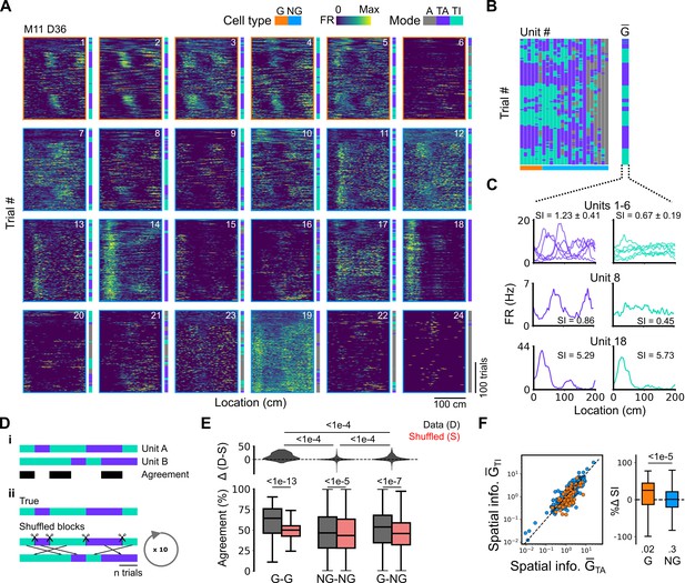
Grid cells and non-grid cells switch between coding schemes coherently.
(A) Joint activity of 6 simultaneously recorded grid cells (orange frames) and 18 non-grid cells (blue frames) from a single session. For each cell, the firing rate map across trials (left) is shown next to the trial classification (right). (B) Classifications for all grid cells (GC) and non-grid cells (NG) as shown in (A), ordered by their agreement to the most common classification within the recorded network at any particular trial. The common classification for recorded grid cells is shown as . (C) Mean firing rate as a function of position for exemplar units from (A) when was task-anchored (left) and task-independent (right). (D) Strategy for assessing agreement between cells in their firing mode (i) and for generating shuffled datasets (ii). (E) Agreement in the firing mode between each combination of grid (G) and non-grid (NG) cells and corresponding scores for the shuffled data (lower), and the difference between the shuffled and actual scores (upper). Agreement was greater between grid cell pairs than between pairs involving non-grid cells (ANOVA: G-G, p<1e-13, Χ2=58.89, DF =1, NG-NG, p<1e-5, Χ2=20.42, DF =1, G-NG, p<1e-7, Χ2=30.37, DF =1; pairwise comparisons: G-G vs NG-NG, p<1e-4, T=–10.455, DF =10,720, G-G vs G-NG, p<1e-4, T=–8.415, DF =10,710, NG-NG vs G-NG, p<1e-4, T=–6.853, DF =10,352). (F) Spatial information of individual cells during trials in which is task-independent as a function of spatial information during trials in which is task-anchored (left). The difference in spatial information between sessions classed as task-anchored or task-independent on the basis of grid cell activity was greater for grid than non-grid cells (right, ANOVA: p<1e-5, Χ2=21.1, DF =1; G vs zero, p=0.018, T=2.723, DF =11.87; NG vs zero, p=0.3, T=–1.278, DF =2.58). The percentage change in spatial information was calculated as .
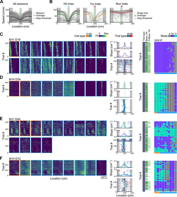
Spatial behaviour during task-anchored and task-independent grid modes.
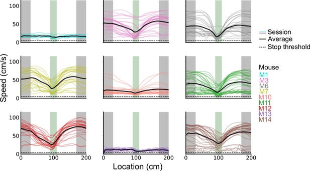
(A) Averages across each behavioural session of running speeds as a function of track position for all sessions. (B) Running speed as a function of track position for trial outcomes classified as hit, try, or run for an example session. (C–F) Examples of variation in the behaviour-related activity of grid and non-grid cells recorded on the location memory task, illustrating firing patterns that are stable and task-anchored (C) or task-independent (D) firing, and unstable firing where cells switch between task-anchored and task-independent modes (E–F). Plots show all simultaneously recorded cells’ firing rate maps in each session (left), stop rasters (lower centre), stop density on beaconed (B) and non-beaconed (NB) trials coloured according to whether grid cells were task-anchored or task-independent (upper centre) and a summary of raster of behaviour and cell classifications (right). Shaded regions in stop density plots represent standard error of the mean measured across epochs. The number of trials classified in a particular coding scheme is also provided with the stop density plot. Grid cells and non-grid cells are colour-coded by bounding boxes around the firing rate map.

Classification of trial outcomes.
Trials were classified into hits, tries, and runs, based on stopping locations and the speed profile on a given trial. First, trials were classified into hits and misses based on whether a stop was registered in the reward zone or not. Next, a distribution of the average speeds in the reward zone is drawn for hit and miss trials, the 95th percentile of the hit average speeds in the reward zone was used to split the miss trials into near hits (tries) and run-throughs (runs). Finally, trials in which the mouse’s average speed outside of the reward zone was <10 cm/s were removed to better discriminate trial outcomes based on the mouse’s engagement.
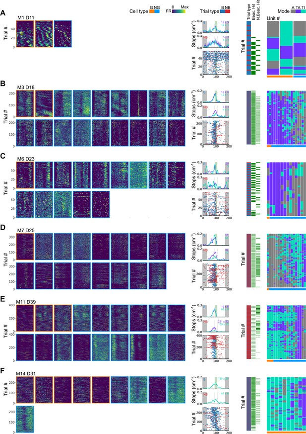
Further examples of spatial behaviour during task-anchored and task-independent grid modes.
(A–F) Examples of variation in the behaviour-related activity of grid and non-grid cells recorded on the location memory task. Plots show all simultaneously recorded cells’ firing rate maps in each session (left), stop rasters (lower centre), stop density on beaconed (B) and non-beaconed (NB) trials coloured according to whether grid cells were task-anchored or task-independent (upper centre) and a summary of raster of behaviour and cell classifications (right). Shaded regions in stop density plots represent standard error of the mean measured across epochs. The number of trials classified in a particular coding scheme is also provided with the stop density plot. Grid cells and non-grid cells are colour-coded by bounding boxes around the firing rate map.
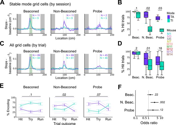
Anchoring of grid firing to the task reference frame promotes localisation by path integration but is not required for cued localisation.
(A, C) Stopping probability relative to baseline as a function of position for sessions with stable grid codes (A) and for epochs within sessions containing both stable and unstable codes (C). Shaded regions in A and C represent standard error of the mean measured across sessions and epochs respectively. N represents the number of sessions with stable codes (A) and the number of grid cells with coding epochs (C). Stable sessions were defined as a session with at least one grid cell for which >85% of trials were in a single coding mode. (B, D) Percentage of hits on beaconed, non-beaconed, and probe trials when the code is task-anchored or task-independent for (B) sessions with stable codes (ANOVA: beaconed, p=0.1, Χ2=2.70, DF=1; non-beaconed, p=0.022, Χ2=5.24, DF=1; probe, p=0.033, Χ2=4.55, DF=1) and when epochs within sessions are task-anchored or task-independent (D) (ANOVA: beaconed, p=0.09, Χ2=2.84, DF=1; non-beaconed, p=0.001, Χ2=10.14, DF=1; probe, p=0.19, Χ2=1.70, DF=1, see Materials and methods). (E) Percentage of trials with hit, try, and run outcomes in which grid cell firing is task-anchored (TA) or task-independent (TI) (ANOVA: beaconed, p=0.11, Χ2=4.49, DF=2; non-beaconed, p=0.02, Χ2=7.75, DF=2; probe, p=0.07, Χ2=5.40, DF=2). Error bars denote standard error of the mean measured across the mean values for each animal. Faded lines show percentage values for individual mice that contained hit, try, and run trials for a given trial type. (F) Odds ratio between receipt of reward for trials on which epochs contain task-anchored firing relative to trials on which epochs contain task-independent firing (beaconed-G, p=0.23; non-beaconed-G, p=0.001; probe-G, p=0.27).
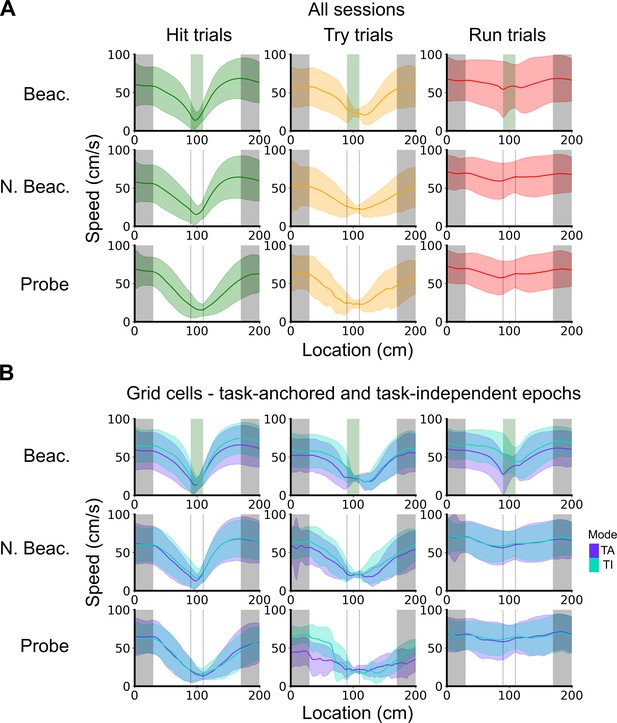
Speed profiles across different trial outcomes.
(A) Running speed as a function of track location for all combinations of trial types and trial outcomes. Shaded regions represent standard deviations measured across trials. (B) Same as in A, however trials were subdivided further based on the coding scheme of grid cells. In cases where multiple grid cells were recorded simultaneously, the same trial was used multiple times to calculate the average speed profile.
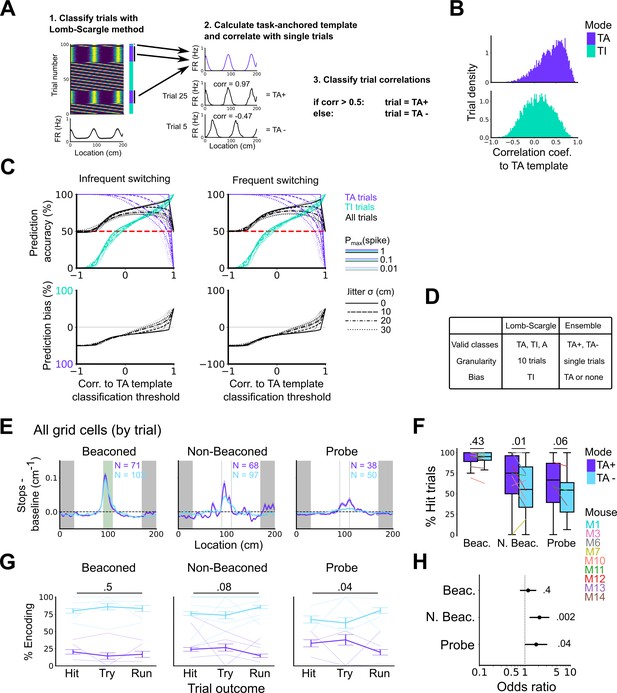
High correlation to the task-anchoring template of grid firing promotes localisation by path integration but is not required for cued localisation.
(A) Procedure for classifying trials using an ensemble method (Lomb-Scargle+template correlation). (B) Trial density of all trial template correlations for trials classified as task-anchored (upper) or task-independent (bottom) using the Lomb-Scargle method. The same trial may be represented multiple times based on the number of simultaneously recorded cells. (C) To assess classification accuracy using the ensemble method, we calculated the prediction accuracy and bias of simulated grid cells (see Materials and methods). Chance level is denoted with a red dashed line. Plots on the left show the prediction accuracy (top) and the prediction bias (bottom) when grid cells alternate between task-anchored and task-independent firing fields in blocks of trials (as in i, iii above), whereas the right plots show the same information for a higher switching frequency (as in ii, iv above). (D) Summary table detailing the pros and cons of each method. (E) Stopping probability relative to baseline as a function of position for epochs within sessions containing both stable and unstable codes. Shaded regions represent standard error of the mean measured across epochs. N represents the number of grid cells with coding epochs. (F) Percentage of hits on beaconed, non-beaconed, and probe trials when the code is task-anchored or task-independent for epochs within sessions are task-anchored or task-independent (ANOVA: beaconed, p=0.43, Χ2=0.62, DF=1; non-beaconed, p=0.01, Χ2=6.43, DF=1; probe, p=0.06, Χ2=3.52, DF=1). (G) Percentage of trials with hit, try, and run outcomes in which grid cell firing is highly correlated with task-anchored firing (ANOVA: beaconed, p=0.51, Χ2=1.35, DF=2; non-beaconed, p=0.08, Χ2=5.14, DF=2; probe, p=0.04, Χ2=6.67, DF=2). Error bars denote standard error of the mean measured across the mean values for each animal. Faded lines show percentage values for individual mice that contained hit, try, and run trials for a given trial type. (H) Odds ratio between receipt of reward for trials on which epochs contain task-anchored firing relative to trials on which epochs contain task-independent firing (beaconed, p=0.4; non-beaconed, p=0.002; probe, p=0.04).

Plot shows the grid field distribution during stable grid cell session (> 85 % task-anchored or task-independent) (A) or during task-anchored and task-independent trials (B).
Shaded regions in A and B represent standard error of the mean measured across sessions and epochs respectively.
Tables
| Reagent type (species) or resource | Designation | Source or reference | Identifiers | Additional information |
|---|---|---|---|---|
| Strain, strain background (mouse) | C57BL/6 | In-house breeding | NA | NA |
| Software, algorithm | R | NA | 4.2.3 | https://www.r-project.org/ |
| Software, algorithm | Python | NA | 3.8.1 | https://www.python.org/ |
| Software, algorithm | ImageJ | Fiji | NA | https://fiji.sc |
| Software, algorithm | Blender | NA | 2.7 | https://www.blender.org/ |
| Software, algorithm | Open Ephys | NA | 0.4.4 | https://open-ephys.org/ |
| Software, algorithm | CTAn | NA | 1.13.5.1 | NA |
| Other | EIB-16 | NeuralLynx | Cat# 31-0603-0106 | NA |
| Other | Platinum/Iridium wire | NeuralLynx | NA | NA |
| Other | Gold Plating Solution | 20 ml Gold Plating Solution | NA | |
| Other | Headpost | RIVETS | NA | https://dudmanlab.org/html/rivets.html |
| Other | UV curing dental cement | RelyX | Cat# 56874 | https://www.3m.co.uk/3M/en_GB/p/d/b00007450/ |
| Other | Simplex Rapid | Kemdent | Cat# ACR803 | https://www.kemdent.co.uk/simplex-rapid-powder-clear-225g?osCsid=j0b5160aallnl2kcdtjpas4oj1 |
| Other | Omnetics to Mill-Max adaptor | Axona | HSADPT-NN1 | NA |
| Other | RHD 6 ft ultrathin SPI cable | Intan | Cat# C3206 | https://open-ephys.org/ |
| Other | RHD 6 ft standard SPI cable | Intan | Cat# C3218 | https://intantech.com/ |
| Other | Acquisition board | Open Ephys | NA | https://open-ephys.org/ |
Additional files
-
Supplementary file 1
Summary table of recorded cells and estimated tetrode locations.
- https://cdn.elifesciences.org/articles/89356/elife-89356-supp1-v1.docx
-
MDAR checklist
- https://cdn.elifesciences.org/articles/89356/elife-89356-mdarchecklist1-v1.docx
-
Source data 1
MicroCT imaging for tetrode localisation 1/2.
- https://cdn.elifesciences.org/articles/89356/elife-89356-data1-v1.png
-
Source data 2
MicroCT imaging for tetrode localisation 2/2.
- https://cdn.elifesciences.org/articles/89356/elife-89356-data2-v1.png


