Figures and data in An emerging view of neural geometry in motor cortex supports high-performance decoding

Figures
Tables
Additional files

8 figures, 9 tables and 1 additional file

Figures

Figure 1

Download asset Open asset

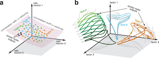
Two perspectives on the structure of neural activity during motor tasks.

(a) Illustration of a traditional perspective. Each neural state (*colored dots*) is an N-dimensional vector of firing rates. States are limited to a manifold that can be usefully approximated by a subspace. In this illustration, neural states are largely limited to a two-dimensional subspace within the full three-dimensional firing-rate space. Within that restricted subspace, there exist neural dimensions where neural activity correlates with to-be-decoded variables. BCI decoding leverages knowledge of the subspace and of those correlations. If two tasks have similar motor outputs at two particular moments, the corresponding neural states will also be similar, aiding generalization. (b) An emerging perspective. Neural activity is summarized by neural factors (one per axis), with each neuron’s firing rate being a simple function of the factors. Factors may be numerous (many dozens or even hundreds), resulting in a high-dimensional subspace of neural activity. Yet most of that space is unoccupied; factor-trajectories are heavily constrained by the underlying dynamics (*gray arrows*), such that most states are never visited. The order in which states are visited is also heavily sculpted by dynamics; e.g. trajectories rarely ‘swim upstream’. The primary constraint is thus not a subspace, but a sparse manifold where activity largely flows in specific directions. Different tasks may often (but not always) employ different dynamics and thus different regions of the manifold. Because most aspects of neural trajectories fall in the null space of outgoing commands, there are no directions in neural state space that consistently correlate with kinematic variables, and distant states may correspond to similar motor outputs.

Figure 2

Download asset Open asset

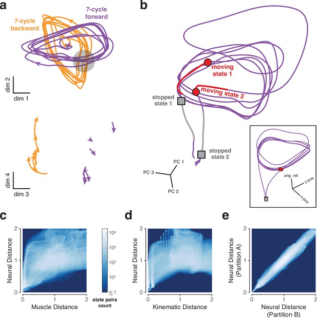
Properties of neural trajectories in motor cortex, illustrated for data recorded during the cycling task (MC_Cycle dataset).

(a) Low tangling implies separation between trajectories that might otherwise be close. *Top*. Neural trajectories for forward (*purple*) and backward (*orange*) cycling. Trajectories begin 600 ms before movement onset and end 600 ms after movement offset. Trajectories are based on trial-averaged firing rates, projected onto two dimensions. Dimensions were selected to highlight apparent crossings of the cyclic trajectories during forward and backward cycling, while also capturing considerable variance (11.5%, comparable to the 11.6% captured by PCs 3 and 4). *Gray region* highlights one set of apparent crossings. *Bottom*. Trajectories during the restricted range of times in the gray region, but projected onto different dimensions. The same scale is used in top and bottom subpanels. (b) Examples of well-separated neural states (*main panel*) corresponding to similar behavioral states (*inset*). Colored trajectory tails indicate the previous 150 ms of states. Data from 7-cycle forward condition. (c) Joint distribution of pairwise distances for muscle and neural trajectories. Analysis considered all states across all conditions. For both muscle and neural trajectories, we computed all possible pairwise distances across all states. Each muscle state has a corresponding neural state, from the same time within the same condition. Thus, each pairwise muscle-state distance has a corresponding neural-state distance. The color of each pixel indicates how common it was to observe a particular combination of muscle-state distance and neural-state distance. Muscle trajectories are based on 7 z-scored intramuscular EMG recordings. Correspondence between neural and muscle state pairs included a 50 ms lag to account for physiological latency. Results were not sensitive to the presence or size of this lag. Neural and muscle distances were normalized (separately) by average pairwise distance. (d) Same analysis for neural and kinematic distances (based on phase and angular velocity). Correspondence between neural and kinematic state pairs included a 150 ms lag. Results were not sensitive to the presence or size of this lag. (e) Control analysis to assess the impact of sampling error. If two sets of trajectories (e.g. neural and kinematic) are isometric and can be estimated perfectly, their joint distribution should fall along the diagonal. To estimate the impact of sampling error, we repeated the above analysis comparing neural distances across two data partitions, each containing 15–18 trials/condition.

Figure 3

Download asset Open asset

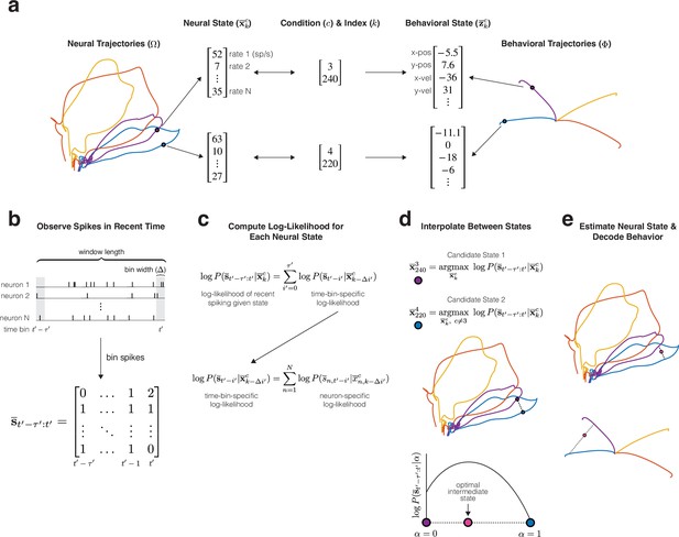
Example training (*top panel*) and decoding (*bottom panels*) procedures for MINT, illustrated using four conditions from a reaching task.

(a) Libraries of neural and behavioral trajectories are learned such that each neural state ${\bar{x}}_{k}^{c}$ corresponds to a behavioral state ${\bar{z}}_{k}^{c}$ . (b) Spiking observations are binned spike counts (20 ms bins for all main analyses). ${\bar{s}}_{t^{'} - τ^{'} : t^{'}}$ contains the spike count of each neuron for the present bin, $t^{'}$ , and $τ^{'}$ bins in the past. (c) At each time step during decoding, the log-likelihood of observing ${\bar{s}}_{t^{'} - τ^{'} : t^{'}}$ is computed for each and every state in the library of neural trajectories. Log-likelihoods decompose across neurons and time bins into Poisson log-likelihoods that can be queried from a precomputed lookup table. A recursive procedure (not depicted) further improves computational efficiency. (d) Two candidate neural states (*purple* and *blue*) are identified. The first is the state within the library of trajectories that maximizes the log-likelihood of the observed spikes. The second state similarly maximizes that log-likelihood, with the restriction that the second state must not come from the same trajectory as the first (i.e. must be from a different condition). Interpolation identifies an intermediate state that maximizes log-likelihood. (e) The optimal interpolation is applied to candidate neural states – yielding the final neural-state estimate – and their corresponding behavioral states – yielding decoded behavior. Despite utilizing binned spiking observations, neural and behavioral states can be updated at millisecond resolution (Methods).

Figure 4 with 1 supplement

Download asset Open asset

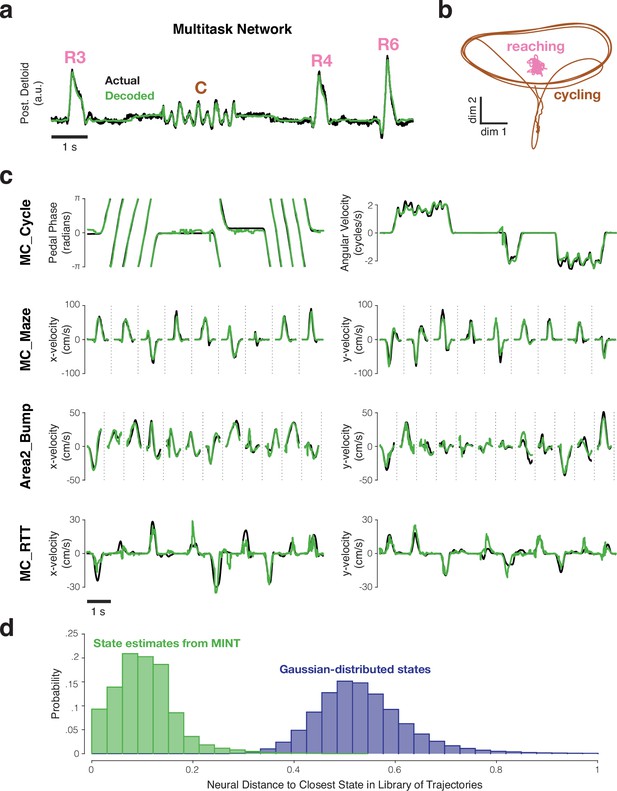
Examples of behavioral decoding provided by MINT for one simulated dataset and four empirically recorded datasets.

All decoding is causal; only spikes from before the decoded moment are used. (a) MINT was applied to spiking data from an artificial spiking network. That network was trained to generate posterior deltoid activity and to switch between reaching and cycling tasks. Based on spiking observations, MINT approximately decoded the true network output at each moment. ‘R3’, ‘R4’, and ‘R6’ indicate three different reach conditions. ‘C’ indicates a cycling bout. MINT used no explicit task-switching, but simply tracked neural trajectories across tasks as if they were conditions within a task. (b) Illustration of the challenging nature, from a decoding perspective, of network trajectories. Trajectories are shown for two dimensions that are strongly occupied during cycling. Trajectories for the 8 reaching conditions (*pink*) are all nearly orthogonal to the trajectory for cycling (*brown*) and thus appear compressed in this projection. (c) Decoded behavioral variables (*green*) compared to actual behavioral variables (*black*) across four empirical datasets. MC_Cycle and MC_RTT show 10 seconds of continuous decoding. MC_Maze and Area2_Bump show randomly selected trials, demarcated by *vertical dashed lines*. (d) Distribution of distances between each decoded neural state and the nearest state in the library $Ω$ (*green*), for the MC_Cycle dataset. To provide a reference, we drew neural states from a Gaussian distribution whose mean and covariance matched the library states, and computed distances to the library states (*purple*). This emulates what would occur if the manifold were defined by the data covariance and associated neural subspace. The *green* distribution mostly contains non-zero values, but is much closer to zero than the *purple* distribution. Thus, MINT rarely decodes a neural state that exactly matches a library state, but most decoded states are close to the scaffolding provided by the library states. Neural distances are normalized by the average pairwise distance between library states.

Figure 4—video 1

Download asset

posterframe for video — Video demonstrating causal neural state estimation and behavioral decoding from MINT on the MC_Cycle dataset.

In this dataset, a monkey moved a hand pedal cyclically forward or backward in response to visual cues. The raster plot of spiking activity (112 neurons, *bottom right subpanel*) and the actual and decoded angular velocities of the pedal (*top right subpanel*) are animated with 10 seconds of trailing history. Decoding was causal; the decode of the present angular velocity (right hand edge of scrolling traces) was based only on present and past spiking. Cycling speed was ∼2 Hz. The underlying neural state estimate (*green sphere in left subpanel*) is plotted in a 3D neural subspace, with a 2D projection below. The present neural state is superimposed on top of the library of 8 neural trajectories used by MINT. The state estimate always remained on or near (via state interpolation) the neural trajectories. *Purple* and *orange* trajectories correspond to forward and backward cycling conditions, respectively. The lighter-to-darker color gradients differentiate between trajectories corresponding to 1-, 2-, 4-, and 7-cycle conditions for each cycling direction. Neural state estimate corresponds in time to the right edge of the scrolling raster/velocity plot. The three-dimensional neural subspace was hand-selected to capture a large amount of neural variance (59.6%; close to the 62.9% captured by the top 3 PCs) while highlighting the dominant translational and rotational structure in the trajectories.

Figure 5 with 2 supplements

Download asset Open asset

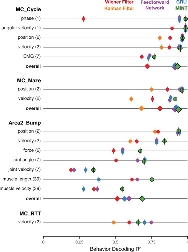
Comparison of decoding performance, for MINT and four additional algorithms, for four datasets and multiple decoded variables.

On a given trial, MINT decodes all behavioral variables in a unified way based on the same inferred neural state. For non-MINT algorithms, separate decoders were trained for each behavioral group (with the exception of the Kalman filter, which used the same model to decode position and velocity). E.g. separate GRUs were trained to output position and velocity in MC_Maze. Parentheticals indicate the number of behavioral variables within a group. E.g. ‘position (2)’ has two components: x- and y-position. $R^{2}$ is averaged across behavioral variables within a group. ‘Overall’ plots performance averaged across all behavioral groups. $R^{2}$ values for feedforward networks and GRUs are additionally averaged across runs for 10 random seeds. The Kalman filter is traditionally utilized for position- and velocity-based decoding and was therefore only used to predict these behavioral groups. Accordingly, the ‘overall’ category excludes the Kalman filter for datasets in which the Kalman filter did not contribute predictions for every behavioral group. Results are based on the following numbers of training / test trials: MC_Cycle (174 train, 99 test), MC_Maze (1721 train, 574 test), Area2_Bump (272 train, 92 test), MC_RTT (810 train, 268 test). Vertical offsets and vertical ticks are used to increase visibility of data when symbols overlap.

Figure 5—figure supplement 1

Download asset Open asset

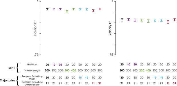
MINT’s decoding performance is robust to the choice of hyperparameters.

MINT was run on the MC_Maze dataset with systematic perturbations to two of MINT’s hyperparameters: bin width (ms) and window length (ms). Bin width is the size of the bin in which spikes are counted: 20 ms for all analyses in the main figures. Window length is the length, in milliseconds, of spiking history that is considered. For all main analyses of the MC_Maze dataset, this was 300 ms, i.e. MINT considered the spike count in the present bin and in 14 previous bins. Perturbations were also made to two hyperparameters related to learning neural trajectories: temporal smoothing width (standard deviation of Gaussian filter applied to spikes) and condition-smoothing dimensionality (see Methods). These two hyperparameters describe how aggressively the trial-averaged data are smoothed (across time and conditions, respectively) when learning rates. Baseline decoding performance (*black circles*) was computed using the same hyperparameters that were used with the MC_Maze dataset in the analyses from Figures 4 and 5. Then, decoding performance was computed by perturbing each of the four hyperparameters twice (*colored circles*): once to ∼50% of the hyperparameter’s baseline value and once to ∼150%. Trials were bootstrapped (1000 resamples) to generate 95% confidence intervals (*error bars*). Perturbations of hyperparameters had little impact on performance. Altering bin width had essentially no impact, nor did altering temporal smoothing. Shortening window length had a negative impact, presumably because MINT had to estimate the neural state using fewer observations. However, the drop in performance was minimal: $R^{2}$ dropped by .011 for position decoding only. Reducing the number of dimensions used for across-condition smoothing, and consequently over-smoothing the data, had a negative impact on both position and velocity decoding. Yet again this was small: e.g. velocity $R^{2}$ dropped by .010. These results demonstrate that MINT can achieve high performance using hyperparameter values that span a large range. Thus, they do not need to be meticulously optimized to ensure good performance. In general, optimization may not be needed at all, as MINT’s hyperparameters can often be set based on first principles. For example, in this study, bin width was never optimized either for specific datasets or in general. We chose to always count spikes in 20 ms bins (except in the perturbations shown here) because this duration is long enough to reduce computation time yet short relative to the timescales over which rates change. Additionally, window length can be optimized (as we did for decoding analyses), but it could also simply be chosen to roughly match the timescale over which past behavior tends to predict future behavior. Temporal smoothing of trajectories when building the library can simply use the same values commonly used when analyzing such data. For example, in prior studies, we have used smoothing kernels of width 20–30 ms when computing trial-averaged rates, and these values also support excellent decoding. Condition smoothing is optional and need not be applied at all, but may be useful if one wishes to record fewer trials for more conditions. For example, rather than record 15 trials for 8 reach directions, one might wish to record 5 trials for 24 conditions, then use condition smoothing to reduce sampling error.

Figure 5—figure supplement 2

Download asset Open asset

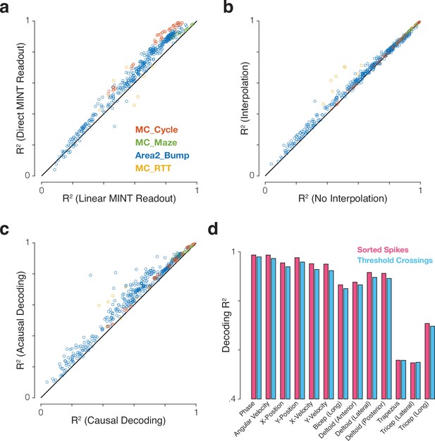
Impact of different modeling and preprocessing choices on performance of MINT.

For most applications we anticipate MINT will employ direct decoding that leverages the correspondence between neural and behavioral trajectories, but one could also choose to linearly decode behavior from the estimated neural state. For most applications, we anticipate MINT will use interpolation amongst candidate neural states on neighboring trajectories, but one could also restrict decoding to states within the trajectory library. For real-time applications we anticipate MINT will be run causally, but acausal decoding (using both past and future spiking observations) could be used offline or even online by introducing a lag. We anticipate MINT may be used both in situations where spike events have been sorted based on neuron identity, and situations where decoding simply uses channel-specific unsorted threshold crossings. Panels (**a-c**) explore the first three choices. Performance was quantified for all eight combinations of: direct MINT readout vs. linear MINT readout, interpolation vs. no interpolation, causal decoding vs. acausal decoding. This was done for 121 behavioral variables across four datasets for a total of 964 $R^{2}$ values. The ‘phase’ behavioral variable in MC_Cycle was excluded from ‘linear MINT readout’ variants because its circularity makes it a trivially poor target for linear decoding. (a) MINT’s direct neural-to-behavioral-state association outperforms a linear readout based on MINT’s estimated neural state. Performance was significantly higher using the direct readout ( $Δ R^{2}$ =0.061 ± 0.002 SE; p<0.001, paired t-test). Note that the linear readout still benefits from the ability of MINT to estimate the neural state using all neural dimensions, not just those that correlate with kinematics. (b) Decoding with interpolation significantly outperformed decoding without interpolation ( $Δ R^{2}$ =0.018 ± 0.001 SE; p<0.001, paired t-test). (c) Running acausally significantly improved performance relative to causal decoding ( $Δ R^{2}$ =0.051 ± 0.002 SE; p<0.001, paired t-test). Although causal decoding is required for real-time applications, this result suggests that (when tolerable) introducing a small decoding lag could improve performance. For example, a decoder using 200 ms of spiking activity could introduce a 50 ms lag such that the decode at time $t$ is rendered by generating the best estimate of the behavioral state at time $t - 50$ using spiking data from $t - 200$ through $t$ . (d) Decoding performance for 13 behavioral variables in the MC_Cycle dataset when sorted spikes were used (112 neurons, *pink*) versus ‘good’ threshold crossings from electrodes for which the signal-to-noise ratio of the firing rates exceeded a threshold (93 electrodes, SNR >2, *cyan*). The loss in performance when using threshold crossings was small ( $Δ R^{2}$ =–0.014 ± 0.002 SE). SE refers to standard error of the mean.

Figure 6 with 1 supplement

Download asset Open asset

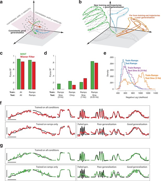
Implications of neural geometry for decoder generalization, in principle and in practice.

(a) Under a traditional perspective, training that explores the full range of to-be-decoded variables will also explore the relevant neural manifold, allowing future generalization. *Gray dots* indicate neural states observed during training. *Colored traces* indicate newly observed trajectories. Because these trajectories traverse the previously defined manifold, they can be decoded by leveraging the established correlations between manifold dimensions and kinematics. (b) Under an emerging perspective, generalization is possible when new trajectories lie within a similar region of factor-space as training-set trajectories. *Gray-dashed traces* indicate training-set neural trajectories. *Colored traces* indicate newly observed trajectories. *Green* and *blue* trajectories largely follow the flow-field implied by training-set trajectories, allowing generalization. In contrast, the *orange* trajectory evolves far from any previously explored region, challenging generalization. This may occur even when behavioral outputs overlap with those observed during training. (c) Basic decoding performance on the MC_PacMan task for MINT (*green*) and a Wiener filter (*red*). Test sets used held-out trials from the same conditions as training sets. Force-decoding was excellent both when considering all conditions and when considering only ramps (fast and slow, increasing and decreasing). Results are based on the following numbers of training and test trials: All (234 train, 128 test), Ramps (91 train, 57 test). (d) Generalization when training employed the four ramp conditions and testing employed a sine or chirp. Results are based on 91 training trials (all cases) and the following numbers of test trials: Ramps (57), 0.25 Hz Sine (19), 1 Hz Sine (12), 3 Hz Sine (15), Chirp (25). (e) Data likelihoods indicate strained generalization. We computed the log-likelihood of the spiking observations for each neural state decoded by MINT. Rightward values indicate that those observations were unlikely even for the state selected as most likely to have generated those observations. Training employed the four ramp conditions. Distributions are shown when test data employed ramps, a 0.25 Hz sine, or a 3 Hz sine. (f) Examples of force decoding traces (for held-out trials) when decoding using the Wiener filter. *Top row:* all conditions were used during training. *Bottom row:* training employed the four ramp conditions. Horizontal and vertical scale bars correspond to 2 s and 16 Newtons, respectively. (g) As above, but when decoding using MINT. Trials and scale bars are matched across (f) and (g). Representative trials were selected as those that achieved median decoding performance by MINT within each condition.

Figure 6—figure supplement 1

Download asset Open asset

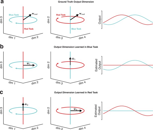
Illustration of why decoding will typically fail to generalize across tasks when neural trajectories occupy orthogonal subspaces.

In theory, learning the output-potent dimensions in motor cortex would be an effective strategy for biomimetic decoding that generalizes to novel tasks. In practice, it is difficult (and often impossible) to statistically infer these dimensions without observing the subject’s full behavioral repertoire (at which point generalization is no longer needed because all the relevant behaviors were directly observed). (a) In this toy example, two neural trajectories occupy fully orthogonal subspaces. In the ‘blue task’, the neural trajectory occupies dimensions 1 and 2. In the ‘red task’, the neural trajectory occupies dimensions 3 and 4. Trajectories in both subspaces have a non-zero projection onto $w_{o u t}$ , enabling neural activity from each task to drive the appropriate output. The output at the right is simply the projection of the blue-task and red-task trajectories onto $w_{o u t}$ . (b) Illustration of the difficulty of inferring $w_{o u t}$ from only one task. In this example, $w_{o u t}$ is estimated using data from the blue task, by linearly regressing the observed output against the neural trajectory for the blue task. The resulting estimate, ${\hat{w}}_{1}$ , correctly translates neural activity in the blue task into the appropriate time-varying output, but fails to generalize to the red task. This failure to generalize is a straightforward consequence of the fact that ${\hat{w}}_{1}$ was learned from data that didn’t explore dimensions 3 and 4. Note that this same phenomenon would occur if ${\hat{w}}_{1}$ were estimated by regressing intended output versus neural activity (as might occur in a paralyzed patient). (c) Estimating the output-potent dimension based only on the red task yields an estimate, ${\hat{w}}_{2}$ , that fails to generalize to the blue task. This phenomenon is illustrated here for a linear readout, but would apply to most nonlinear methods as well, unless some additional form of knowledge allows inferences regarding neural trajectories in previously unseen dimensions.

Figure 7

Download asset Open asset

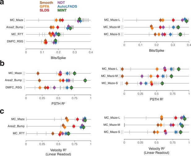
Evaluation of neural state estimates for seven datasets.

(a) Performance quantified using bits per spike. The benchmark’s baseline methods have colored markers. All other submissions have gray markers. Vertical offsets and vertical ticks are used to increase visibility of data when symbols are close due to similar values. Results with negative values are designated by markers to the left of zero, but their locations don’t reflect the magnitude of the negative values. Data from Neural Latents Benchmark (https://neurallatents.github.io/). (b) Performance quantified using PSTH $R^{2}$ . (c) Performance quantified using velocity $R^{2}$ , after velocity was decoded linearly from the neural state estimate. A linear decode is used simply as a way of evaluating the quality of neural state estimates, especially in dimensions relevant to behavior.

Figure 8 with 2 supplements

Download asset Open asset

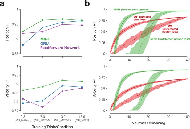
Decoding robustness in the face of small training sets and reduced neuron counts.

(a) $R^{2}$ values for MINT and two neural network decoders (GRU and the feedforward network) when decoding position and velocity for four maze datasets with progressively fewer training trials per condition. Results are based on the following numbers of training and testing trials: MC_Maze-S (75 train, 25 test), MC_Maze-M (188 train, 62 test), MC_Maze-L (375 train, 125 test), MC_Maze (1721 train, 574 test). MC_Maze contains 108 conditions and the other maze datasets each contain 27 conditions. (b) Decoding performance in the face of undetected (*dashed traces*) and known (*solid traces*) loss of neurons. $R^{2}$ values are shown for MINT (*green*) and the Wiener filter (*red*) when decoding position and velocity from the MC_Maze-L dataset (same train/test trials as in a). To simulate undetected neuron loss, we chose $k$ neurons (randomly, with $k$ being the number of lost neurons out of 162 total) and eliminated their spikes without adjusting the decoders. This procedure was repeated 50 times for each value of $k$ . Traces show the mean and standard deviation of the sampling distribution (equivalent to the standard error). To simulate known neuron loss, we followed the above procedure but altered the decoder to account for the known loss. For MINT, this simply involved ignoring the lost neurons when computing data likelihoods. In contrast, the Wiener filter had to be retrained using training data with those neurons eliminated (as would be true for most methods). This was done separately for each set of lost neurons.

Figure 8—figure supplement 1

Download asset Open asset

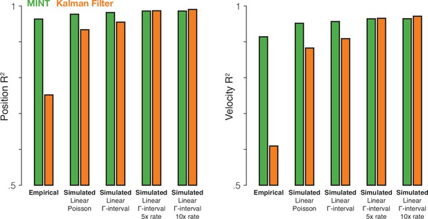
The Kalman filter’s relative performance would improve if neural data had different statistical properties.

We compared MINT to the Kalman filter across one empirical dataset (MC_Maze) and four simulated datasets (same behavior as MC_Maze, but simulated spikes). Simulated firing rates were linear functions of hand position, velocity, and acceleration (as is assumed by the Kalman filter). The means and standard deviations (across time and conditions) of the simulated firing rates were matched to actual neural data (with additional rate scaling in two cases). The Kalman filter assumes that observation noise is stationary and Gaussian. Although spiking variability cannot be Gaussian (spike counts must be positive integers), spiking variability can be made more stationary by letting that variability depend less on rate. Thus, although the first simulation generated spikes via a Poisson process, subsequent simulations utilized gamma-interval spiking (gamma distribution with $α = 2$ and $β = 2 λ$ , where $λ$ is firing rate). Gamma-interval spiking variability of this form is closer to stationary at higher rates. Thus, the third and fourth simulations scaled up firing rates to further push spiking variability into a more stationary regime at the expense of highly unrealistic rates (in the fourth simulation, a firing rate briefly exceeded 1800 Hz). Overall, as the simulated neural data better accorded with the assumptions of the Kalman filter, decoding performance for the Kalman filter improved. Interestingly, MINT continued to perform well even on the simulated data, likely because MINT can exploit a linear relationship between neural and behavioral states when the data argue for it and higher rates benefit both algorithms. These results demonstrate that algorithms like MINT and the Kalman filter are not intrinsically good or bad. Rather, they are best suited to data that match their assumptions. When simulated data approximate the assumptions of the Kalman filter, both methods perform similarly. However, MINT shows much higher performance for the empirical data, suggesting that its assumptions are a better match for the statistical properties of the data.

Figure 8—figure supplement 2

Download asset Open asset

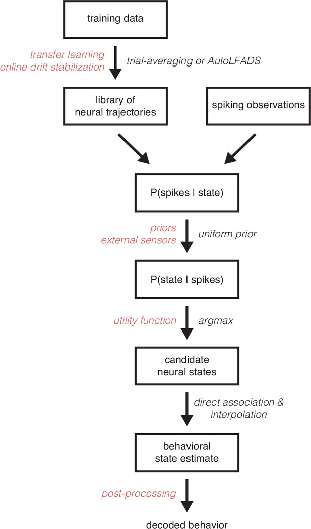
MINT is a modular algorithm amenable to a variety of modifications and extensions.

The flowchart illustrates the standard MINT algorithm in *black* and lists potential changes to the algorithm in *red*. For example, the library of neural trajectories is typically learned via standard trial-averaging or a single-trial rate estimation technique like AutoLFADS. However, transfer learning could be utilized to learn the library of trajectories based on trajectories from a different subject or session. The trajectories could also be modified online while MINT is running to reflect changes in spiking activity that relate to recording instabilities. A potential modification to the method also occurs when likelihoods are converted into posterior probabilities. Typically, we assume a uniform prior over states in the library. However, that prior could be set to reflect the relative frequency of different behaviors and could even incorporate time-varying information from external sensors (e.g. state of a prosthetic limb, eye tracking, etc.) that include information about how probable each behavior is at a given moment. Another potential extension of MINT occurs at the stage where candidate neural states are selected. Typically, these states are selected based solely on spike count likelihoods. However, one could use a utility function that reflects a user’s values (e.g. the user may dislike some decoding mistakes more than others) in conjunction with the likelihoods to maximize expected utility. Lastly, the behavioral estimate that MINT returns could be post-processed (e.g. temporally smoothed). MINT’s modularity largely derives from the fact that the library of neural trajectories is finite. This assumption enables posterior probabilities to be directly computed for each state, rather than analytically derived. Thus, choices like how to learn the library of trajectories, which observation model to use (e.g. Poisson vs. generalized Poisson), and which (if any) state priors to use, can be made independently from one another. These choices all interact to impact performance. Yet they will not interact to impact tractability, as would have been the case if one analytically derived a continuous posterior probability distribution.

Tables

Table 1

MINT training times and average execution times (average time it took to decode a 20 ms bin of spiking observations).

To be appropriate for real-time applications, execution times will ideally be shorter than the bin width. Note that the 20 ms bin width does not prevent MINT from decoding every millisecond; MINT updates the inferred neural state and associated behavioral state between bins, using neural and behavioral trajectories that are sampled every millisecond. For all table entries (except MC_RTT training time), means and standard deviations were computed across 10 train/test runs for each dataset. Training times exclude loading datasets into memory and any hyperparameter optimization. Timing measurements taken on a Macbook Pro (on CPU) with 32GB RAM and a 2.3 GHz 8-Core Intel Core i9 processor. Training and execution code used for timing measurements was written in MATLAB (with the core recursion implemented as a MEX file). For MC_RTT, training involved running AutoLFADS twice (and averaging the resulting rates) to generate neural trajectories. This training procedure utilized 10 GPUs and took ∼1.6 hr per run. For AutoLFADS, hyperparameter optimization and model fitting procedures are intertwined. Thus, the training time reported includes time spent optimizing hyperparameters.

Dataset	Training Time (s)	Execution Time (ms)
Area2_Bump	4.8 ± 0.2	0.31 ± 0.03
MC_Cycle	20.3 ± 2.9	0.55 ± 0.03
MC_Maze	42.8 ± 0.6	2.26 ± 0.09
MC_Maze-L	10.8 ± 0.4	0.83 ± 0.02
MC_Maze-M	8.0 ± 0.4	0.80 ± 0.04
MC_Maze-S	5.8 ± 0.2	0.59 ± 0.07
MC_RTT	∼3.2 hr	6.99 ± 0.28

Table 2

Neuron, condition, and trial counts for each dataset.

For some datasets, there are additional trials that are excluded from these counts. These trials are excluded because they were only usable for Neural Latents Benchmark submissions due to hidden behavioral data and partially hidden spiking data (see “Neural Latents Benchmark” section).

Dataset	Neurons	Conditions	Trials
Area2_Bump	65	16	364
DMFC_RSG	54	40	1006
MC_Cycle	112	8	273
MC_Maze	182	108	2295
MC_Maze-L	162	27	500
MC_Maze-M	152	27	250
MC_Maze-S	142	27	100
MC_RTT	130	N/A	1080
MC_PacMan	128	8	362
Maze Simulations	182	108	2295
Multitask Network	1200	9	270

Table 3

Hyperparameters for learning neural trajectories via standard trial-averaging.

$σ$ is the standard deviation of the Gaussian kernel used to temporally filter spikes. Trial-averaging Type I and Type II procedures are described in the “Averaging across trials” section. $D_{n e u r a l}$ and $D_{c o n d i t i o n}$ are the neural- and condition-dimensionalities described in the “Smoothing across neurons and/or conditions” section. ‘Full’ means that no dimensionality reduction was performed. Condition smoothing could not be performed for MC_Cycle or the multitask network because different conditions in these datasets are of different lengths (i.e. $K_{c}$ is not the same for all $c$ ). (C) and (R) refer to the cycling and reaching trajectories, respectively, in the multitask network. $t_{m o v e}$ , $t_{s t o p}$ , and $t_{g o}$ correspond to movement onset, movement offset, and the ‘go’ time in the ready-set-go task, respectively. In MC_PacMan, each force profile is padded with static target forces at the beginning and end. $t_{p r o f_s t a r t}$ and $t_{p r o f_e n d}$ mark the beginning and end of the non-padded force profile on each trial.

Dataset	Trajectory Start	Trajectory End	$σ$	Trial Averaging	$D_{n e u r a l}$	$D_{c o n d i t i o n}$
Area2_Bump	$t_{m o v e}$ – 350	$t_{m o v e}$ + 750	25	Type II	Full	Full
DMFC_RSG	$t_{g o}$ – 1950	$t_{g o}$ + 750	55	Type I	49	17
MC_Cycle	$t_{m o v e}$ – 600	$t_{s t o p}$ + 600	30	Type I	Full	N/A
MC_Maze	$t_{m o v e}$ – 500	$t_{m o v e}$ + 700	30	Type II	Full	21
MC_Maze-L	$t_{m o v e}$ – 500	$t_{m o v e}$ + 700	35	Type II	Full	16
MC_Maze-M	$t_{m o v e}$ – 500	$t_{m o v e}$ + 700	60	Type II	Full	20
MC_Maze-S	$t_{m o v e}$ – 500	$t_{m o v e}$ + 700	85	Type II	120	10
MC_PacMan	$t_{p r o f_s t a r t}$ – 1000	$t_{p r o f_e n d}$ + 1000	35	Type II	Full	Full
Maze Simulations	$t_{m o v e}$ – 500	$t_{m o v e}$ + 700	30	Type II	Full	21
Multitask Network	(C) $t_{m o v e}$ – 1000 (R) $t_{m o v e}$ – 800	(C) $t_{s t o p}$ + 1000 (R) $t_{m o v e}$ + 1000	15	Type I	Full	N/A

Table 4

Details for decoding analyses.

The number of training and testing trials for each dataset are provided along with the evaluation period over which performance was computed. Generalization analyses used subsets of these training and testing trials. The window lengths refer to the amount of spiking history MINT used for decoding (e.g. when $τ^{'} = 14$ and $Δ = 20$ the window length is $(τ^{'} + 1) Δ = 300$ ms). $t_{m o v e}$ corresponds to movement onset, $t_{s t o p}$ corresponds to movement offset, $t_{s t a r t}$ refers to the beginning of a trial, and $t_{e n d}$ refers to the end of a trial. There is no defined condition structure for MC_RTT to use for defining trial boundaries. Thus, each trial is simply a 600 ms segment of data, with no alignment to movement. Although 270 of these segments were available for testing, the first 2 segments lacked sufficient spiking history for all decoders to be evaluated and were therefore excluded, leaving 268 test trials. In MC_PacMan, each force profile is padded with static target forces at the beginning and end. $t_{p r o f_s t a r t}$ and $t_{p r o f_e n d}$ mark the beginning and end of the non-padded force profile on each trial. For the multitask network, performance was evaluated on a continuous stretch of 135 trials spanning ∼7.1 minutes.

Dataset	Training Trials	Test Trials	Evaluation Start	Evaluation End	Window Length (ms)
Area2_Bump	272	92	$t_{m o v e}$ – 100	$t_{m o v e}$ + 500	240
MC_Cycle	174	99	$t_{m o v e}$ – 250	$t_{s t o p}$ + 250	200
MC_Maze	1721	574	$t_{m o v e}$ – 250	$t_{m o v e}$ + 450	300
MC_Maze-L	375	125	$t_{m o v e}$ – 250	$t_{m o v e}$ + 450	300
MC_Maze-M	188	62	$t_{m o v e}$ – 250	$t_{m o v e}$ + 450	300
MC_Maze-S	75	25	$t_{m o v e}$ – 250	$t_{m o v e}$ + 450	340
MC_RTT	810	268	$t_{s t a r t}$	$t_{s t a r t}$ + 599	480
MC_PacMan	234	128	$t_{p r o f_s t a r t}$ – 500	$t_{p r o f_e n d}$ + 1000	300
Maze Simulations	1721	574	$t_{m o v e}$ – 250	$t_{m o v e}$ + 450	300
Multitask Network	135	135	$t_{s t a r t}$ (first trial)	$t_{e n d}$ (last trial)	300

Table 5

Details for neural state estimation results.

Note that the training trial counts match the total number of trials reported in Table 2. This reflects that the Neural Latents Benchmark utilized an additional set of test trials not reflected in the Table 2 trial counts. The test trials used for this analysis have ground truth behavior hidden by the benchmark creators and are therefore only suitable for this analysis.

Dataset	Training Trials	Test Trials	Held-in Neurons	Held-out Neurons	Window Length (ms)
Area2_Bump	364	98	49	16	500
DMFC_RSG	1006	283	40	14	1500
MC_Maze	2295	574	137	45	500
MC_Maze-L	500	100	122	40	500
MC_Maze-M	250	100	114	38	500
MC_Maze-S	100	100	107	35	500
MC_RTT	1080	271	98	32	500

Appendix 1—table 1

Hyperparameters used for the Wiener filter.

The L2 regularization term $λ$ was optimized in the range [0, 2000], with the optimized values rounded to the closest multiple of 10. Window lengths were optimized (in 20 ms increments) in the range [200, 600] for Area2_Bump, [200, 1000] for MC_Cycle, [200, 1200] for MC_RTT, [200, 500] for MC_PacMan, and [200, 700] for MC_Maze, MC_Maze-L, MC_Maze-M, and MC_Maze-S. These ranges were determined by the structure of each dataset (e.g. Area2_Bump couldn’t look back more than 600 ms from the beginning of the evaluation epoch without entering the previous trial). Window lengths are directly related to $κ$ via $Δ$ (e.g. $κ = 14$ would correspond to a window length of $Δ (κ + 1) = 20 (14 + 1) = 300$ ms).

Dataset	Behavioral Group	Window Length (ms)	L2 Regularization (λ)
Area2_Bump	Position	560	350
	Velocity	320	320
	Force	600	900
	Joint Angles	300	250
	Joint Velocities	400	1410
	Muscle Lengths	380	0
	Muscle Velocities	460	940
MC_Cycle	Phase	1000	1730
	Angular Velocity	960	1470
	Position	920	1710
	Velocity	420	600
	EMG	560	1990
MC_Maze	Position	660	530
MC_Maze	Velocity	540	210
MC_Maze-L	Position	540	510
MC_Maze-L	Velocity	540	440
MC_Maze-M	Position	660	440
MC_Maze-M	Velocity	480	310
MC_Maze-S	Position	680	130
MC_Maze-S	Velocity	420	270
MC_RTT	Velocity	1180	1610
MC_PacMan	Force	480	470

Appendix 1—table 2

Hyperparameters used for the Kalman filter.

The lag (in increments of 20 ms time bins) between neural activity and behavior was optimized in the range [2, 8], corresponding to 40–160 ms, for all datasets except Area2_Bump. For Area2_Bump the lag was not optimized and was simply set to 0 due to the fact that, in a sensory area, movement precedes sensory feedback. Given that $x_{k}$ aggregates spikes across the whole time bin, but $y_{k}$ corresponds to the behavioral variables at the end of the time bin, the effective lag is actually half a bin (10 ms) longer — i.e. the effective range of lags considered for the non-sensory datasets was 50–170 ms.

Dataset	Behavioral Group	Lag (bins)
Area2_Bump	Position & Velocity	0
MC_Cycle	Position & Velocity	2
MC_Maze	Position & Velocity	4
MC_Maze-L	Position & Velocity	4
MC_Maze-M	Position & Velocity	4
MC_Maze-S	Position & Velocity	4
MC_RTT	Position & Velocity	2

Appendix 1—table 3

Hyperparameters used for the feedforward neural network.

The number of hidden layers ( $L$ ) was optimized in the range [1, 15]. The number of units per hidden layer ( $D$ ) was optimized in the range [50, 1000], with the optimized values rounded to the closest multiple of 10. The dropout rate was optimized in the range [0,0.5] and the number of training epochs was optimized in the range [2, 100]. Window lengths were optimized (in 20 ms increments) in the range [200, 600] for Area2_Bump, [200, 1000] for MC_Cycle, [200, 1200] for MC_RTT, and [200, 700] for MC_Maze, MC_Maze-L, MC_Maze-M, and MC_Maze-S.

Dataset	Behavioral Group	Window Length (ms)	Hidden Layers (L)	Units/Layer (D)	Dropout Rate	Epochs
Area2_Bump	Position	440	4	690	0.20	58
	Velocity	520	5	260	0	62
	Force	240	4	560	0.01	54
	Joint Angles	320	7	480	0.15	59
	Joint Velocities	460	5	660	0.12	36
	Muscle Lengths	240	10	840	0.19	81
	Muscle Velocities	500	6	480	0.02	24
MC_Cycle	Phase	740	8	180	0.11	24
	Angular Velocity	700	8	710	0.01	43
	Position	360	9	470	0	45
	Velocity	460	5	330	0.25	55
	EMG	840	5	970	0.07	43
MC_Maze	Position	680	7	340	0.15	65
MC_Maze	Velocity	700	14	760	0	89
MC_Maze-L	Position	380	6	160	0.05	44
MC_Maze-L	Velocity	600	8	380	0.13	43
MC_Maze-M	Position	520	8	860	0.26	79
MC_Maze-M	Velocity	420	2	360	0.09	59
MC_Maze-S	Position	580	8	340	0.02	74
MC_Maze-S	Velocity	520	4	210	0.07	94
MC_RTT	Velocity	1040	2	700	0.15	17

Appendix 1—table 4

Hyperparameters used for the GRU network.

The number of units ( $D$ ) was optimized in the range [500, 1000], with the optimized values rounded to the closest multiple of 10. The dropout rate was optimized in the range [0,0.5] and the number of training epochs was optimized in the range [2, 50]. Window lengths were optimized (in 20 ms increments) in the range [200, 600] for Area2_Bump, [200, 1000] for MC_Cycle, [200, 1200] for MC_RTT, and [200, 700] for MC_Maze, MC_Maze-L, MC_Maze-M, and MC_Maze-S.

Dataset	Behavioral Group	Window Length (ms)	Units (D)	Dropout Rate	Epochs
Area2_Bump	Position	560	700	0.06	12
	Velocity	340	820	0.32	3
	Force	380	380	0.27	26
	Joint Angles	480	630	0.31	8
	Joint Velocities	260	390	0.27	9
	Muscle Lengths	460	990	0.34	45
	Muscle Velocities	420	870	0.19	47
MC_Cycle	Phase	460	580	0.18	49
	Angular Velocity	480	390	0.12	27
	Position	920	760	0.06	42
	Velocity	520	170	0.43	45
	EMG	840	250	0.40	36
MC_Maze	Position	640	740	0.27	4
MC_Maze	Velocity	520	800	0.34	11
MC_Maze-L	Position	620	640	0.40	49
MC_Maze-L	Velocity	580	420	0.36	31
MC_Maze-M	Position	620	820	0.41	48
MC_Maze-M	Velocity	660	840	0.29	30
MC_Maze-S	Position	460	310	0.39	27
MC_Maze-S	Velocity	680	500	0.44	45
MC_RTT	Velocity	540	890	0.40	8

Additional files

MDAR checklist: https://cdn.elifesciences.org/articles/89421/elife-89421-mdarchecklist1-v1.pdf
Download elife-89421-mdarchecklist1-v1.pdf

Download links

A two-part list of links to download the article, or parts of the article, in various formats.

Downloads (link to download the article as PDF)

Open citations (links to open the citations from this article in various online reference manager services)

Mendeley

Cite this article (links to download the citations from this article in formats compatible with various reference manager tools)

Sean M Perkins
Elom A Amematsro
John Cunningham
Qi Wang
Mark M Churchland

(2025)

An emerging view of neural geometry in motor cortex supports high-performance decoding

eLife 12:RP89421.

https://doi.org/10.7554/eLife.89421.3

Figures

Two perspectives on the structure of neural activity during motor tasks.

Properties of neural trajectories in motor cortex, illustrated for data recorded during the cycling task (MC_Cycle dataset).

Example training (top panel) and decoding (bottom panels) procedures for MINT, illustrated using four conditions from a reaching task.

Examples of behavioral decoding provided by MINT for one simulated dataset and four empirically recorded datasets.

Video demonstrating causal neural state estimation and behavioral decoding from MINT on the MC_Cycle dataset.

Comparison of decoding performance, for MINT and four additional algorithms, for four datasets and multiple decoded variables.

MINT’s decoding performance is robust to the choice of hyperparameters.

Impact of different modeling and preprocessing choices on performance of MINT.

Implications of neural geometry for decoder generalization, in principle and in practice.

Illustration of why decoding will typically fail to generalize across tasks when neural trajectories occupy orthogonal subspaces.

Evaluation of neural state estimates for seven datasets.

Decoding robustness in the face of small training sets and reduced neuron counts.

The Kalman filter’s relative performance would improve if neural data had different statistical properties.

MINT is a modular algorithm amenable to a variety of modifications and extensions.

Tables

MINT training times and average execution times (average time it took to decode a 20 ms bin of spiking observations).

Neuron, condition, and trial counts for each dataset.

Hyperparameters for learning neural trajectories via standard trial-averaging.

Details for decoding analyses.

Details for neural state estimation results.

Hyperparameters used for the Wiener filter.

Hyperparameters used for the Kalman filter.

Hyperparameters used for the feedforward neural network.

Hyperparameters used for the GRU network.

Additional files

MDAR checklist

Download links

Downloads (link to download the article as PDF)

Open citations (links to open the citations from this article in various online reference manager services)

Cite this article (links to download the citations from this article in formats compatible with various reference manager tools)

Be the first to read new articles from eLife

Share this article

Cite this article

Two perspectives on the structure of neural activity during motor tasks.

Properties of neural trajectories in motor cortex, illustrated for data recorded during the cycling task (MC_Cycle dataset).

Example training (top panel) and decoding (bottom panels) procedures for MINT, illustrated using four conditions from a reaching task.

Examples of behavioral decoding provided by MINT for one simulated dataset and four empirically recorded datasets.

Video demonstrating causal neural state estimation and behavioral decoding from MINT on the MC_Cycle dataset.

Comparison of decoding performance, for MINT and four additional algorithms, for four datasets and multiple decoded variables.

MINT’s decoding performance is robust to the choice of hyperparameters.

Impact of different modeling and preprocessing choices on performance of MINT.

Implications of neural geometry for decoder generalization, in principle and in practice.

Illustration of why decoding will typically fail to generalize across tasks when neural trajectories occupy orthogonal subspaces.

Evaluation of neural state estimates for seven datasets.

Decoding robustness in the face of small training sets and reduced neuron counts.

The Kalman filter’s relative performance would improve if neural data had different statistical properties.

MINT is a modular algorithm amenable to a variety of modifications and extensions.

MINT training times and average execution times (average time it took to decode a 20 ms bin of spiking observations).

Neuron, condition, and trial counts for each dataset.

Hyperparameters for learning neural trajectories via standard trial-averaging.

Details for decoding analyses.

Details for neural state estimation results.

Hyperparameters used for the Wiener filter.

Hyperparameters used for the Kalman filter.

Hyperparameters used for the feedforward neural network.

Hyperparameters used for the GRU network.

MDAR checklist

Downloads (link to download the article as PDF)

Open citations (links to open the citations from this article in various online reference manager services)

Cite this article (links to download the citations from this article in formats compatible with various reference manager tools)