Research Article

Neuroscience

Hippocampus and striatum show distinct contributions to longitudinal changes in value-based learning in middle childhood

Department of Psychology, Goethe University Frankfurt, Germany
Centre for Human Brain Health, School of Psychology, University of Birmingham, United Kingdom
Institute for Mental Health, School of Psychology, University of Birmingham, United Kingdom
Centre for Developmental Science, School of Psychology, University of Birmingham, United Kingdom
Social, Cognitive and Affective Neuroscience Unit, Department of Cognition, Emotion, and Methods in Psychology, Faculty of Psychology, University of Vienna, Austria
Max Planck Research Group Biosocial, Max Planck Institute for Human Development, Germany
Charité – Universitätsmedizin Berlin, Institute of Medical Psychology, Germany
Max Planck School of Cognition, Max Planck Institute for Human Cognitive and Brain Sciences, Germany
Frankfurt Institute for Advanced Studies (FIAS), Germany
Center for Safe & Healthy Children, The Pennsylvania State University, United States

Jul 2, 2024

https://doi.org/10.7554/eLife.89483.3

Open access
Copyright information

Figures
Tables
Additional files

10 figures, 8 tables and 1 additional file

Figures

Figure 1

Download asset Open asset

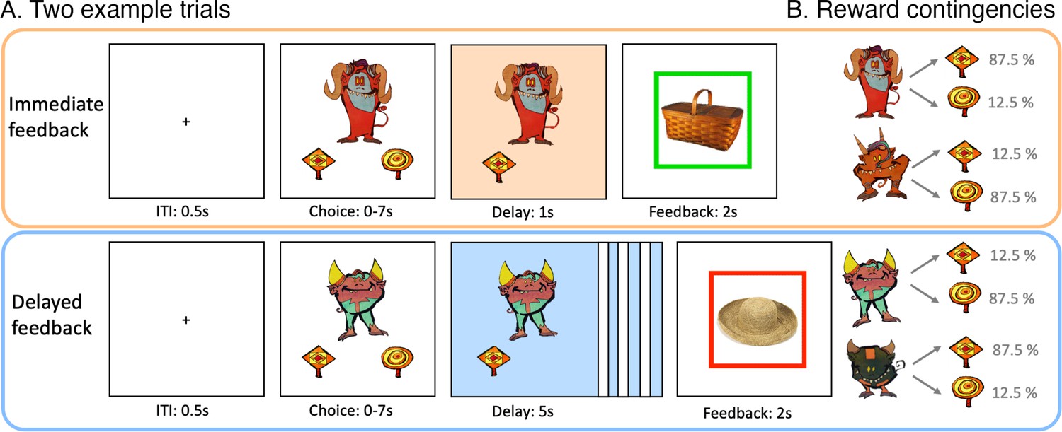
Reinforcement learning task.

(A) Depiction of two example trials of immediate and delayed feedback conditions presented at wave 1. For immediate feedback (top panel), between choice response and feedback, cue and choice were presented for 1 s. At feedback, a green frame around the incidentally encoded object indicated a positive outcome, which appeared in 87.5% of the trials when selecting the squard-shaped lolli for this example cue. For delayed feedback (bottom panel), the delay phase between choice response and feedback lasted for 5 s. The red frame around the object indicated a negative outcome and appeared in 87.5% of the trials when selecting the squard-shaped lolli for this example cue. (B) For each feedback condition, two action-outcome contingencies were learned to balance a potential choice bias. With the four task versions, the cues and outcome contingencies were counterbalanced across participants.

Figure 2

Download asset Open asset

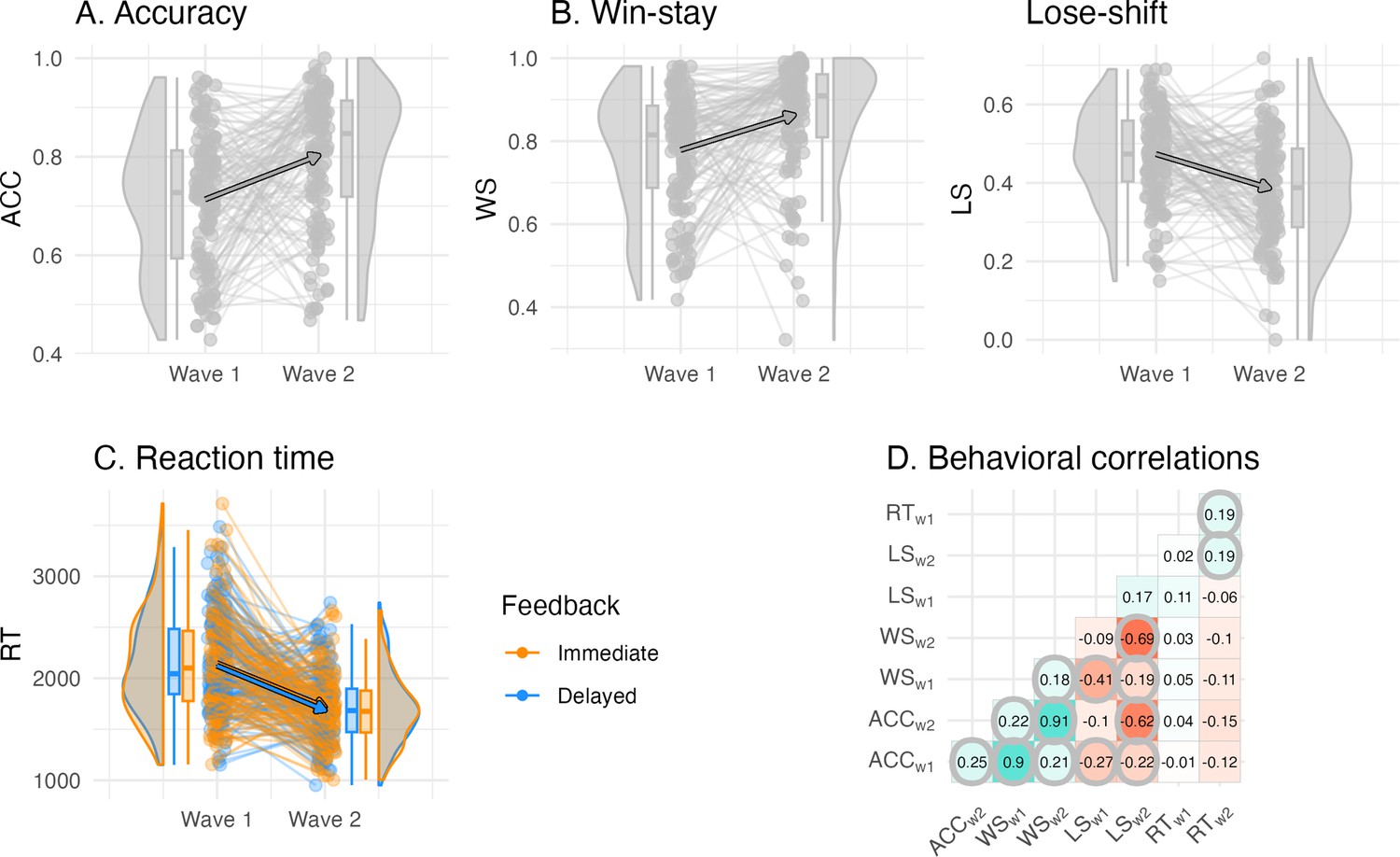
Individual differences in the behavioral learning outcomes and their longitudinal change.

(A) Accuracy did not differ by feedback timing and increased between waves. (B) Win-stay and lose-shift proportion did not differ by feedback timing, and win-stay increased and lose-shift proportion decreased between waves. (C) Reaction time (in ms) differed by feedback timing, in which decisions for cues learned with delayed feedback were faster, and reaction times were faster at wave 2 compared to wave 1. (D) Correlations between behavioral outcomes reveal that learning accuracy was primarily correlated with the win-stay and lose-shift probabilities both within and between waves, but was uncorrelated to reaction time. Significant correlations are circled, p-values were adjusted for multiple comparisons using bonferroni correction.

Figure 3

Download asset Open asset

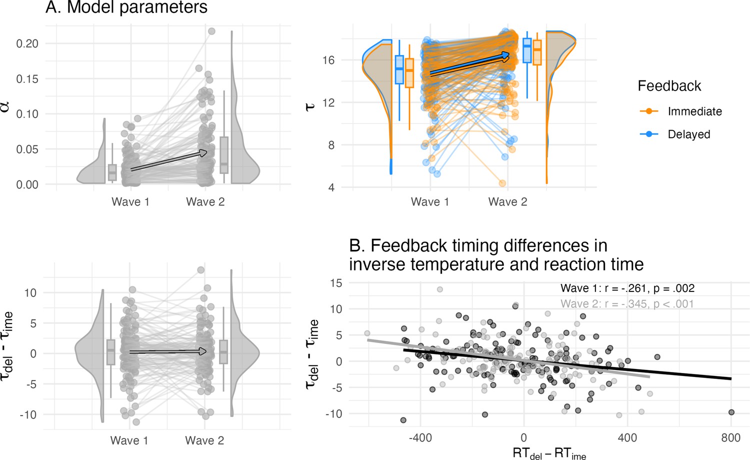
Overview of the computational model parameters.

(A) Individual differences in the learning rate and inverse temperature of the winning model and their longitudinal change. The inverse temperature $τ$ but not learning rate $α$ was separated by feedback timing, and both increased between waves in their values (top panel). The condition difference in the inverse temperature did not differ on average, but showed individual differences (bottom left panel). (B) The condition differences in the inverse temperature correlated with reaction time, that is higher delayed compared to immediate inverse temperature was related to faster delayed compared to immediate reaction time.

Figure 4

Download asset Open asset

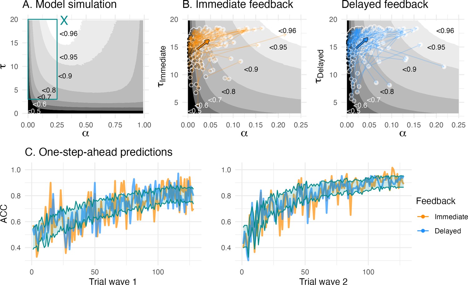
Model simulation/validation.

(A) The model simulation depicts parameter combinations and simulation-based average learning scores. The cyan ‘X’ in the middle top depicts the optimal parameter combination where average learning scores were at 96.5%, and the cyan rectangle depicts the space of the fitted parameter combinations, (B) Enlarged view of the space of fitted parameter combinations. The colored arrows depict mean change (bold arrow) and individual change (transparent arrows) of the fitted parameters. The greyscale gradient-filled dots, that are connected by the arrows, depict the individual learning score, while the the greyscale gradient in the background depicts the simulated average learning score. The mean change reveals an overall change towards the higher, that is, more optimal, learning scores. (C) One-step-ahead posterior predictions of the winning model for each wave. The colored lines depict averaged trial-by-trial task behavior for each feedback condition, and a cyan ribbon indicates the 95% highest density interval of the one-step-ahead prediction using the entire posterior distribution, which included 6000 iterations for each of the 33,460 trials.

Figure 5

Download asset Open asset

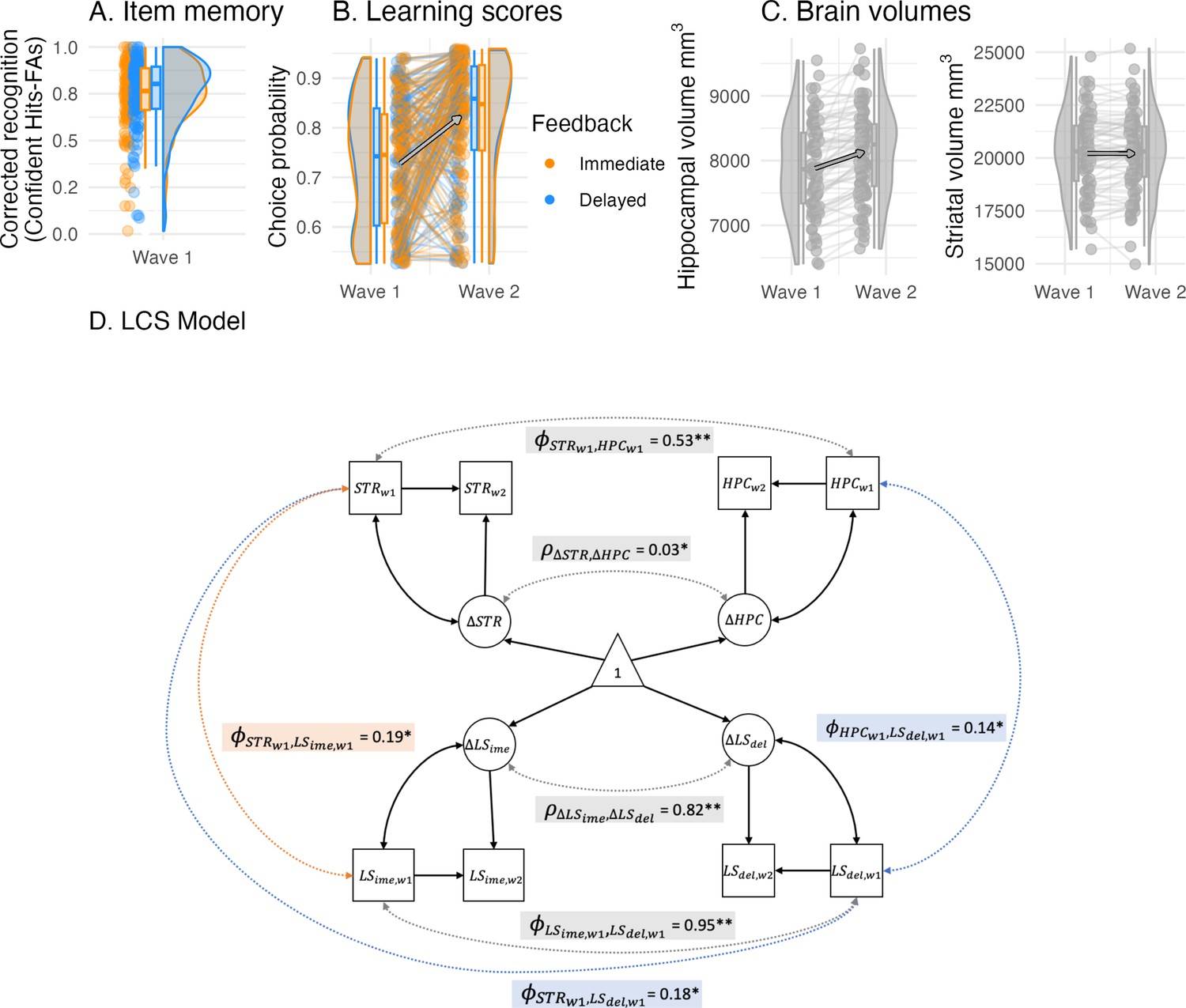
Cognitive and brain measures with cross-sectional and longitudinal links.

(A) Recognition memory (corrected recognition = hits - false alarms) for objects presented during delayed feedback was only enhanced at trend. (B) Learning scores depicted here were used in the LCS analyses. Learning scores were the model-derived choice probability of the contingent choice using fitted posterior parameters. (C) Hippocampal and striatal volumes increased between waves, while hippocampal volume increased most. (D) A four-variate latent change score (LCS) model that included striatal and hippocampal volumes as well as immediate and delayed learning scores. Depicted are significant paths cross-domain (brain-cognition, dashed lines) and within-domain (brain or cognition, solid lines), other paths are omitted for visual clarity and are summarized in Table 4. Depicted brain-cognition links included $ϕ_{{S T R}_{w 1}, {L S}_{i m e, w 1}}$ (covariance between striatal volume and immediate learning score at wave 1), as well as $ϕ_{{H P C}_{w 1}, {L S}_{d e l, w 1}}$ and $ϕ_{{S T R}_{w 1}, {L S}_{d e l, w 1}}$ (covariances between hippocampal and striatal volumes and delayed learning score at wave 1). Brain links included $ϕ_{{S T R}_{w 1}, {H P C}_{w 1}}$ and $ρ_{∆ S T R, ∆ H P C}$ (wave 1 covariance and change-change covariance), and similarly, cognition links included $ϕ_{{L S}_{i m e, w 1}, {L S}_{d e l, w 1}}$ and $ρ_{∆ L S_{i m e}, ∆ L S_{d e l}}$ . Covariates included age, sex and estimated total intracranial volume. ** denotes significance at α < 0.001, * at α < 0.05.

Appendix 1—figure 1

Download asset Open asset

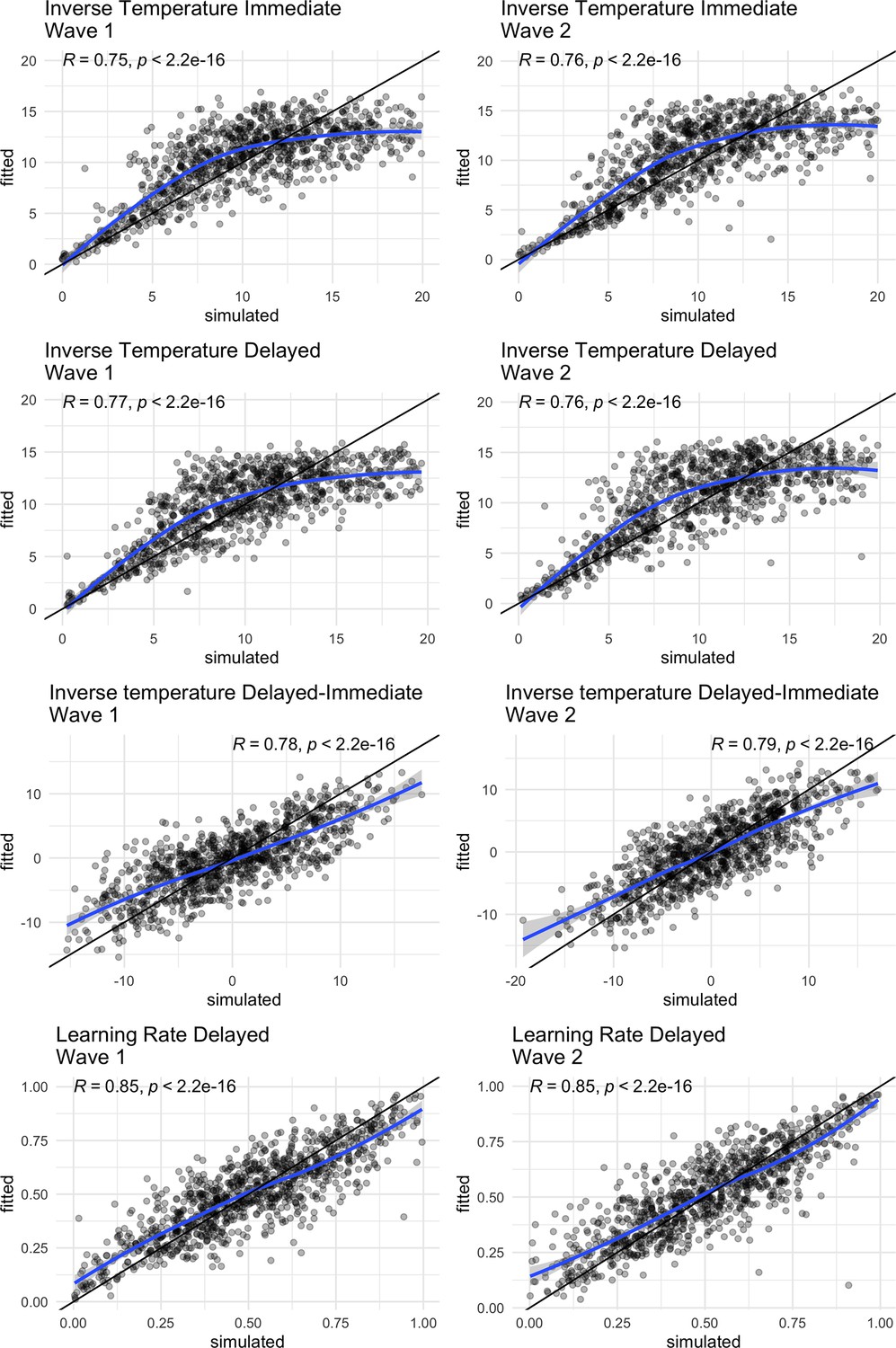
Parameter recovery of the winning model, the black line represents the identity line, whereas the blue line is loess regression line, Correlations are calculated by Pearson’s r.

Appendix 1—figure 2

Download asset Open asset

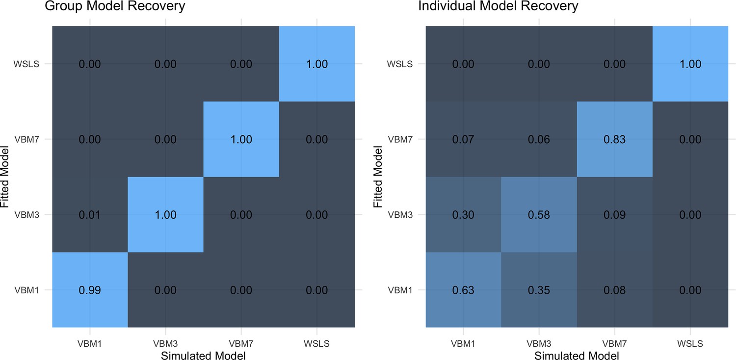
Model recovery on the group (left) and individual level (right).

Group-level recovery values are the average model weights (across 20 groups, 50 datasets each) *Pseudo-BMA*+using Bayesian model averaging stabilized by Bayesian bootstrap using 100,000 iterations. Individual-level recovery values are the average model fits (across 1000 datasets), $e l p d_{l o o}$ which is the individual summed expected log pointwise predictive density of all trials.

Appendix 2—figure 1

Download asset Open asset

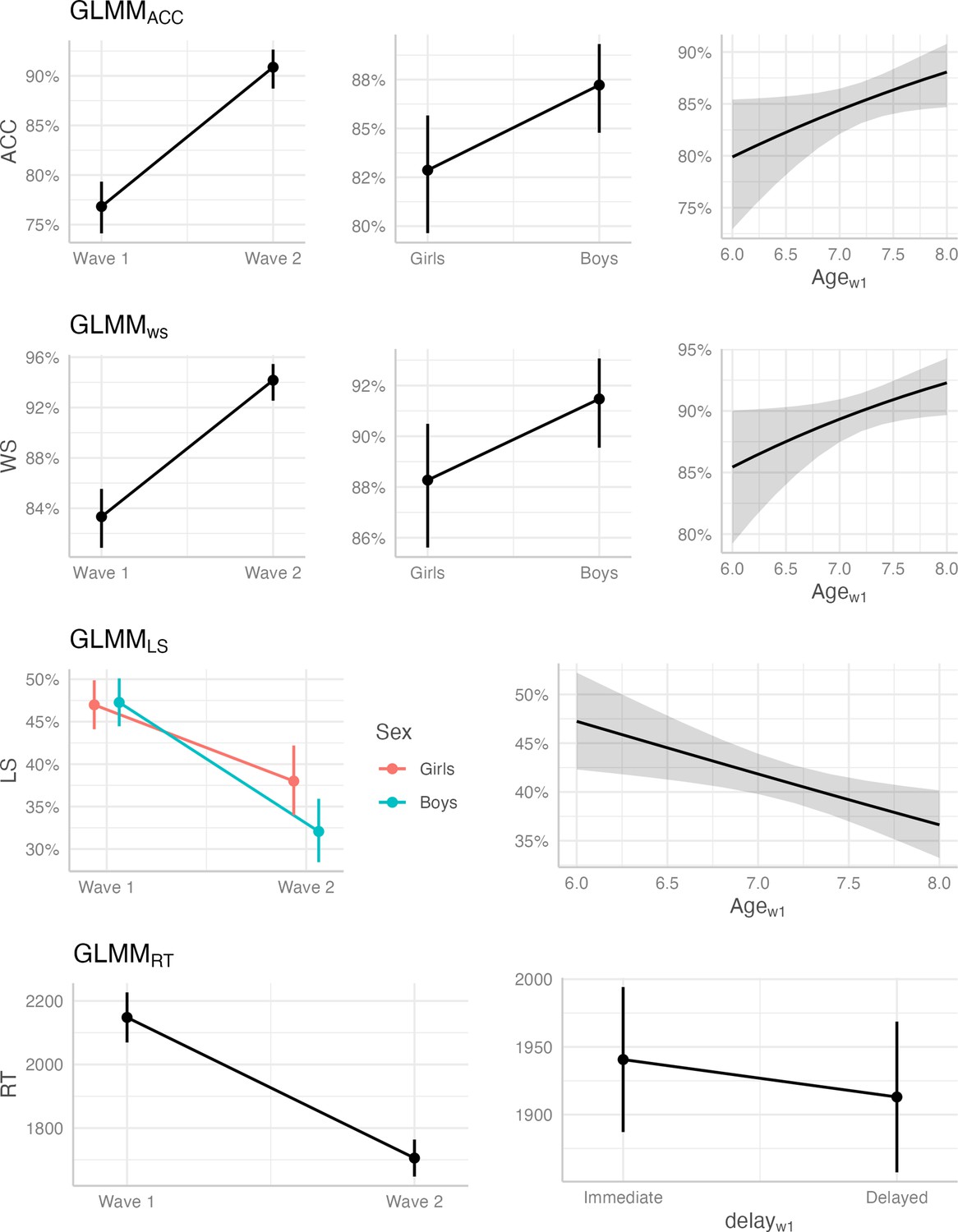
Fixed effects plots of significant predictors across behavioral variables accuracy (ACC), win-stay (WS), lose-shift (LS) and reaction time (RT).

See Appendix 2—table 1 for the statistical results.

Appendix 3—figure 1

Download asset Open asset

Parameter correlations of the winning model.

Significant correlations are circled, p-values were adjusted for multiple comparisons using bonferroni correction.

Appendix 4—figure 1

Download asset Open asset

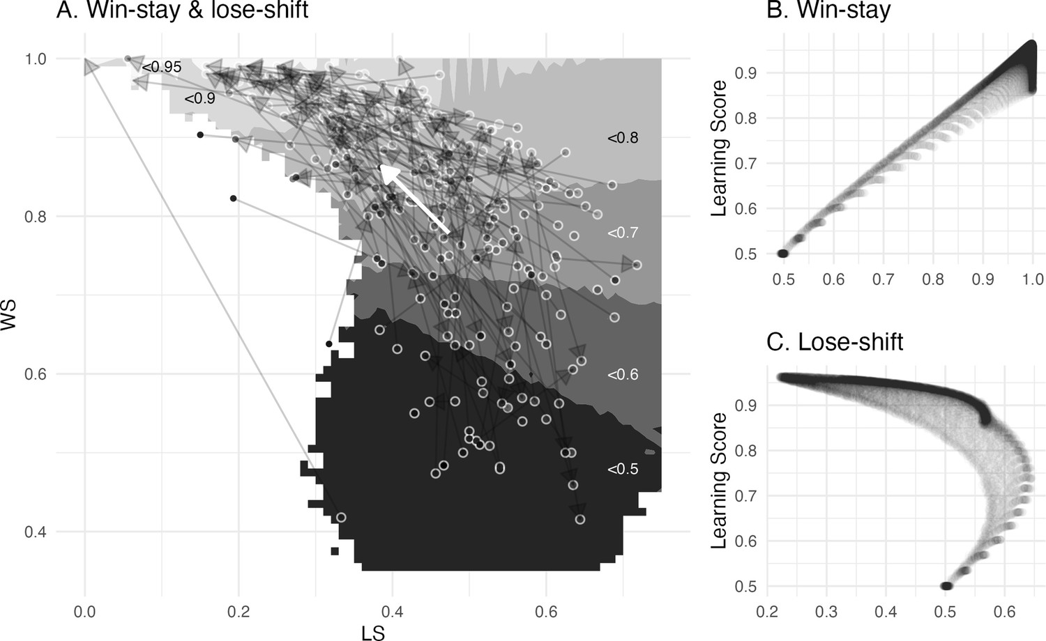
Switching behavior and optimal learning derived from model simulation.

(A) The arrows depict mean change (bold white) and individual change (transparent black) of the empirical win-stay and lose-shift proportions. The greyscale gradient-filled dots, that are connected by the arrows, depict the individual learning score, while the the greyscale gradient in the background depicts the simulated average learning score. The mean change reveals an overall change towards the higher, that is more optimal, learning scores, with higher win-stay and lower lose-shift behavior. (**B, C**) Win-stay and lose-shift behavior plotted against the learning score depict their separate effects on learning optimality. While win-stay showed a positive linear relationship with the learning score, lose-shift showed a negative nonlinear relationship with a larger optimal range.

Tables

Table 1

Behavioral learning outcomes and mixed model fixed effects that predicted the outcomes.

	Descriptive Results				Mixed Model Effects
	Wave 1		Wave 2		Wave	Feedback
	Immediate	Delayed	Immediate	Delayed
ACC	0.69 (0.46)	0.70 (0.46)	0.79 (0.41)	0.80 (0.40)	↑ W2	–
WS	0.81 (0.39)	0.80 (0.40)	0.88 (0.32)	0.88 (0.32)	↑ W2	–
LS	0.47 (0.50)	0.50 (0.50)	0.42 (0.49)	0.42 (0.49)	↓ W2	–
RT	2.10 (1.31)	2.07 (1.29)	1.70 (1.02)	1.67 (1.00)	↓ W2	↓ Delayed

Note. Mean (standard deviation of accuracy) (ACC, probability correct), win-stay probability (WS), lose-shift probability (LS), and reaction time (RT, in seconds), split by wave and feedback timing. Mixed model effects and their directionality of effect (increasing ↑ or decreasing ↓). W2 = Wave 2.

Table 2

Model comparison results.

Model	Parameters	$Δ e l p d_{l o o} [S E]$	$Σ e l p d_{l o o} [m e a n]$	Pseudo-BMA+
Step 1: heuristic strategy models and value-based learning model
$v b m_{1}$	$1 α$ , $1 τ$	0 [0]	–15154.9 [-0.45]	1
$w s$	$1 τ_{w s}$	–1327.7 [159.5]	–16482.7 [-0.49]	< 0.01
$w s l s$	$1 τ_{w s l s}$	–4247.3 [284.8]	–19402.3 [-0.58]	0
Step 2: value-based learning models
$v b m_{3}$	$1 α$ , $2 τ$	0 [0]	–15045.3 [-0.45]	0.73
$v b m_{7}$	$1 α$ , $2 ρ$	–2.93 [2.92]	–15048.2 [-0.45]	0.24
$v b m_{6}$	$2 α$ , $1 ρ$	–24.34 [8.85]	–15069.6 [-0.45]	< 0.01
$v b m_{8}$	$2 α$ , $2 ρ$	–29.71 [15.95]	–15075.0 [-0.45]	0.02
$v b m_{4}$	$2 α$ , $2 τ$	–43.34 [14.89]	–15088.6 [-0.45]	< 0.01
$v b m_{2}$	$2 α$ , $1 τ$	–46.45 [13.97]	–15091.7 [-0.45]	< 0.01
$v b m_{5}$	$1 α$ , $1 ρ$	–59.01 [7.59]	–15104.3 [-0.45]	< 0.01
$v b m_{1}$	$1 α$ , $1 τ$	–109.63 [11.98]	–15154.9 [-0.45]	< 0.01

Note. Model = heuristic ( $w s$ , $w s l s$ ) and value-based models ( $v b m_{1 - 8}$ ) that were compared against each other. Parameters = corresponding model parameters learning rate $α$ , inverse temperature $τ$ and outcome sensitivity $ρ$ . $Δ e l p d_{l o o} [S E]$ = difference in the Bayesian leave-one-out cross-validation estimate of the expected log pointwise predictive density relative to the winning model and its standard errors. $Σ e l p d_{l o o} [m e a n]$ = sum of expected log pointwise predictive density of all 33,460 trials, including all participants and waves, and trial mean. Pseudo-BMA+ = model weight for relative model evidence using Bayesian model averaging stabilized by Bayesian bootstrap with 100,000 iterations.

Table 3

Description of computational model parameters from the winning value-based model $v b m_{3}$ .

	Wave 1					Wave 2
	α	τ_Immediate	τ_Delayed	ls_Immediate	ls_Delayed	α	τ_Immediate	τ_Delayed	ls_Immediate	ls_Delayed
Mean	0.02	14.6	14.8	0.73	0.73	0.05	16.2	16.5	0.82	0.82
SD	0.02	2.04	2.37	0.12	0.13	0.04	2.37	2.21	0.13	0.13
Min	< 0.01	6.73	5.25	0.53	0.53	< 0.01	4.37	6.85	0.53	0.53
Max	0.09	17.5	17.9	0.94	0.94	0.22	18.6	18.7	0.96	0.96

Note. $α$ = learning rate across feedback timing, $τ / l s$ = inverse temperature and learning score separated by conditions of feedback timing.

Table 4

Parameter estimates of a four-variate latent change score model that includes brain (striatal and hippocampal volume) and cognition domains (immediate and delayed learning score).

	$S T R$	${L S}_{i m e}$	$H P C$	${L S}_{d e l}$
Model fit: χ² = 15.4, df = 27, CFI = 1, RMSEA (CI) = 0 (0–0.01), SRMR = 0.045
Mean change Δ	0.06* (0.03)	0.76** (0.08)	0.38** (0.04)	0.75** (0.08)
wave 1 variance σ	fixed to 1	fixed to 1	fixed to 1	fixed to 1
change variance σ_Δ	0.07** (0.01)	0.88** (0.10)	0.18* (0.07)	0.83** (0.10)
Intercept-change regression β	–0.04 (0.04)	–0.83* (0.29)	–0.16* (0.06)	–0.73* (0.27)
Wave 1 covariates
age onto Intercept $ϕ$	0.19 (0.10)	–0.05 (0.08)	0.29* (0.08)	0.08 (0.08)
sex onto Intercept $ϕ$	–0.42** (0.07)	–0.14 (0.07)	–0.47** (0.07)	–0.11 (0.07)
eTIV onto Intercept $ϕ$	0.68** (0.05)	–	0.70** (0.05)	–
Brain-cognition links (cross-domain)	$S T R - L S_{i m e}$	$S T R - L S_{d e l}$	$H P C - L S_{i m e}$	$H P C - L S_{d e l}$
wave 1 covariation $ϕ$	0.19* (0.07)	0.18* (0.07)	0.12 (0.07)	0.14* (0.07)
change-change covariance $ρ$	< 0.01 (0.03)	< 0.01 (0.03)	–0.06 (0.05)	–0.07 (0.05)
wave 1 brain onto cognition change $γ$	0.25 (0.13)	0.22 (0.12)	0.05 (0.11)	0.06 (0.10)
wave 1 cognition onto brain change $γ$	–0.19 (0.13)	0.21 (0.13)	0.05 (0.10)	< 0.01 (0.10)
Brain links (within-domain)	$S T R - H P C$
wave 1 covariation $ϕ$	0.53** (0.07)
change-change covariance $ρ$	0.03* (0.01)
wave 1 striatum onto hippocampal change $γ$	0.06 (0.05)
wave 1 hippocampus onto striatal change $γ$	0.02 (0.03)
Cognition links (within-domain)	$L S_{i m e} - L S_{d e l}$
wave 1 covariation $ϕ$	0.95** (0.10)
change-change covariance $ρ$	0.82** (0.10)
wave 1 ${L S}_{i m e}$ onto ${L S}_{d e l}$ change $γ$	–0.07 (0.27)
wave 1 ${L S}_{d e l}$ onto ${L S}_{i m e}$ change $γ$	0.06 (0.28)

Parameter estimates in bold are the paths of interest depicted in Figure 5D. Standard errors are shown in parentheses. eTIV = estimated total intracranial volume. ** denotes significance at α < 0.001, * at α < 0.05. sex coded as 1 = girls, –1 = boys.

Appendix 2—table 1

Mixed effects model structure and fixed effects results for the models using the dependent variables Accuracy (ACC), win-stay (WS), lose-shift (LS) and Reaction time (RT).

Fixed effects	GLMM_ACC	GLMM_WS	GLMM_LS	GLMM_RT
Feedback = Delayed	0.013	0.023	–0.030	14.0*
Wave = 2	0.550**	0.586**	–0.252**	–218**
Sex = Girls	–0.172*	–0.177*	0.062	23.5
Wave 1 Age	0.142*	0.163*	–0.100*	–24.5
Wave = 1*Sex = Girls	not included	not included	0.068*	not included
Random slopes
Feedback Type	X	X	X	X
Wave	X	X	X	X
Random intercepts
Participant ID	X	X	X	X
Block	X	X	X	X
Model fit
ICC	0.44	0.45	0.12	0.23
Observations	33,460	22,013	10,383	33,460
Marginal R²	0.056	0.063	0.021	0.036
Conditional R²	0.472	0.482	0.138	0.258

Note. ** denotes significance at α < 0.001, * at α < 0.05. X indicates which random effects were included in the final model. ICC = intraclass correlation. Marginal R² = variance explained by fixed effects, Conditional R² = variance explained by fixed and random effects.

Appendix 5—table 1

Model fit and parameter estimates of the univariate LCS models for immediate and delayed feedback learning score as well as for striatal (STR) and hippocampal (HPC) brain volumes.

	${L S}_{i m m e d i a t e}$	${L S}_{d e l a y e d}$	STR	HPC
χ² (df)	1.75 (4)	1.25 (4)	1.61 (6)	1.77 (6)
RMSEA (CI)	0.08 (0–0.08)	0 (0–0.07)	0 (0–0)	0 (0–0.02)
SRMR	0.03	0.03	0.03	0.03
CFI	1.00	1.00	1.00	1.00
Mean change μ_Δ	0.74** (0.09)	0.73** (0.08)	0.06* (0.03)	0.37** (0.05)
w1 variance σ_β	0.99** (0.08)	0.99** (0.07)	0.51** (0.07)	0.46** (0.06)
Change variance σ_Δ	0.94** (0.10)	0.89** (0.10)	0.07** (0.02)	0.18* (0.08)
Intercept-change regression δ	–0.69** (0.08)	–0.73** (0.08)	–0.04 (0.04)	–0.12* (0.04)
Age onto Intercept	–0.07 (0.08)	0.11 (0.08)	0.02 (0.09)	0.15 (0.08)
Sex onto Intercept	–0.20* (0.08)	–0.17* (0.08)	–0.05 (0.09)	–0.09 (0.09)
eTIV onto Intercept	–	–	0.67** (0.09)	0.62** (0.10)

Standard errors in parentheses. ** denotes significance at α < .001, * at α < .05. sex coded as 1 = girls, –1 = boys.

Appendix 6—table 1

Comparison of the fixed effects results for the models with the reduced and with the complete dataset, each with the dependent variables accuracy (ACC), win-stay (WS), lose-shift (LS) and reaction time (RT).

Fixed effects	GLMM_ACC	GLMM_WS	GLMM_LS	GLMM_RT
Reduced dataset (complete dataset)
Feedback = Delayed	0.009 (0.013)	0.022 (0.023)	–0.030 (–0.030)	–16.8* (–13.8*)
Wave = 2	0.492 (0.550)	0.534 (0.586)	–0.252 (–0.252)	–221 (–221)
Sex = Girls	–0.157* (–0.172*)	–0.161* (–0.177*)	0.062 (0.062)	20.6 (20.5)
Wave 1 Age	0.174** (0.142*)	0.186* (0.163*)	–0.100* (–0.100*)	–38.0 (-37.8)
Wave = 1*Sex = Girls	not included	not included	0.068* (0.068*)	not included
Model fit
ICC	0.45 (0.44)	0.45 (0.45)	0.12 (0.12)	0.24 (0.23)
Observations	31857 (33460)	21212 (22013)	10383 (10383)	31857 (33460)
Marginal R²	0.047 (0.056)	0.054 (0.063)	0.024 (0.024)	0.038 (0.036)
Conditional R²	0.473 (0.472)	0.483 (0.482)	0.138 (0.138)	0.266 (0.260)

Note. ** denotes significance at α < 0.001, * at α < 0.05. X indicates which random effects were included in the final model. ICC = intraclass correlation. Marginal R² = variance explained by fixed effects, Conditional R² = variance explained by both fixed and random effects.

Appendix 6—table 2

Model comparison results obtained with the reduced dataset and the complete dataset.

Model	Parameters	Δ𝑒𝑙𝑝𝑑𝑙𝑜𝑜	mean 𝑒𝑙𝑝𝑑𝑙𝑜𝑜	Pseudo-BMA+
Reduced dataset (complete dataset)
step 1: heuristic strategy vs value-based learning model
$v b m_{1}$	$1 α$ , $1 τ$	0 (0)	–0.47 (-0.45)	1 (1)
$w s$	$1 τ_{w s}$	–1296.2 (-1327.7)	–0.51 (-0.49)	0 (< 0.01)
$w s l s$	$1 τ_{w s l s}$	–4164.3 (-4247.3)	–0.61 (-0.58)	0 (0)
step 2: value-based learning model variants
$v b m_{3}$	$1 α$ , $2 τ$	0 (0)	–0.47 (-0.45)	0.78 (0.73)
$v b m_{7}$	$1 α$ , $2 ρ$	–3.71 (-2.93)	–0.47 (-0.45)	0.19 (0.24)
$v b m_{6}$	$2 α$ , $1 ρ$	–24.34 (-24.34)	–0.47 (-0.45)	< 0.01 (< 0.01)
$v b m_{8}$	$2 α$ , $2 ρ$	–29.20 (-29.71)	–0.47 (-0.45)	0.02 (0.02)
$v b m_{4}$	$2 α$ , $2 τ$	–43.86 (-43.34)	–0.47 (-0.45)	< 0.01 (< 0.01)
$v b m_{2}$	$2 α$ , $1 τ$	–45.08 (-46.45)	–0.47 (-0.45)	< 0.01 (< 0.01)
$v b m_{5}$	$1 α$ , $1 ρ$	–57.65 (-59.01)	–0.47 (-0.45)	< 0.01 (< 0.01)
$v b m_{1}$	$1 α$ , $1 τ$	–107.8 (-109.63)	–0.47 (-0.45)	< 0.01 (< 0.01)

Note. Model = Heuristic ( $w s$ , $w s l s$ ) and value-based models ( $v b m_{1 - 8}$ ) that were compared against each other. Parameters = corresponding model parameters learning rate ( $α$ ), inverse temperature ( $τ$ ) and outcome sensitivity ( $ρ$ ). $Δ e l p d_{l o o}$ = differences in Bayesian leave-one-out cross-validation estimate of the expected log pointwise predictive density relative to the winning model and its standard errors. $m e a n e l p d_{l o o}$ = mean of expected log pointwise predictive density across all trials. Pseudo-BMA+ = model weight for relative model evidence using Bayesian model averaging stabilized by Bayesian bootstrap using 100,000 iterations.

Additional files

MDAR checklist: https://cdn.elifesciences.org/articles/89483/elife-89483-mdarchecklist1-v1.docx
Download elife-89483-mdarchecklist1-v1.docx

Download links

A two-part list of links to download the article, or parts of the article, in various formats.

Downloads (link to download the article as PDF)

Article PDF

Open citations (links to open the citations from this article in various online reference manager services)

Mendeley

Cite this article (links to download the citations from this article in formats compatible with various reference manager tools)

Johannes Falck
Lei Zhang
Laurel Raffington
Johannes Julius Mohn
Jochen Triesch
Christine Heim
Yee Lee Shing

(2024)

Hippocampus and striatum show distinct contributions to longitudinal changes in value-based learning in middle childhood

eLife 12:RP89483.

https://doi.org/10.7554/eLife.89483.3

Share this article

Cite this article

Reinforcement learning task.

Individual differences in the behavioral learning outcomes and their longitudinal change.

Overview of the computational model parameters.

Model simulation/validation.

Cognitive and brain measures with cross-sectional and longitudinal links.

Parameter recovery of the winning model, the black line represents the identity line, whereas the blue line is loess regression line, Correlations are calculated by Pearson’s r.

Model recovery on the group (left) and individual level (right).

Fixed effects plots of significant predictors across behavioral variables accuracy (ACC), win-stay (WS), lose-shift (LS) and reaction time (RT).

Parameter correlations of the winning model.

Switching behavior and optimal learning derived from model simulation.

Behavioral learning outcomes and mixed model fixed effects that predicted the outcomes.

Model comparison results.

Description of computational model parameters from the winning value-based model vbm3 .

Parameter estimates of a four-variate latent change score model that includes brain (striatal and hippocampal volume) and cognition domains (immediate and delayed learning score).

Mixed effects model structure and fixed effects results for the models using the dependent variables Accuracy (ACC), win-stay (WS), lose-shift (LS) and Reaction time (RT).

Model fit and parameter estimates of the univariate LCS models for immediate and delayed feedback learning score as well as for striatal (STR) and hippocampal (HPC) brain volumes.

Comparison of the fixed effects results for the models with the reduced and with the complete dataset, each with the dependent variables accuracy (ACC), win-stay (WS), lose-shift (LS) and reaction time (RT).

Model comparison results obtained with the reduced dataset and the complete dataset.

MDAR checklist

Downloads (link to download the article as PDF)

Open citations (links to open the citations from this article in various online reference manager services)

Cite this article (links to download the citations from this article in formats compatible with various reference manager tools)

Description of computational model parameters from the winning value-based model $v b m_{3}$ .