Figures and data in Attention modulates human visual responses to objects by tuning sharpening

Figures
Tables
Additional files

13 figures, 5 tables and 1 additional file

Figures

Figure 1 with 1 supplement

Download asset Open asset

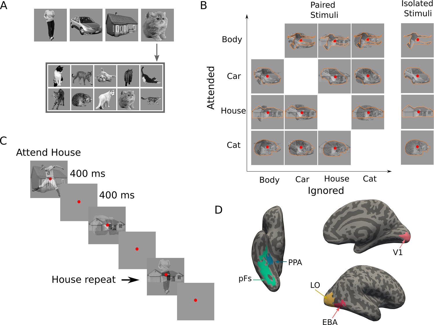
Stimuli, paradigm, and regions of interest.

(A) Top images represent the four categories used in the main experiment: body, car, house, and cat. The stimulus set consisted of 10 exemplars from each category (here: cats), with exemplars differing in pose and 3D-orientation. (B) The experimental design comprised 16 task conditions (12 paired, four isolated). The 4×4 matrix on the left illustrates the 12 paired conditions, with the to-be-attended category (outlined in orange for illustration purposes, not present in the experiment) on the y-axis and the to-be-ignored category on the x-axis. The right column illustrates the four isolated conditions. (C) Experimental paradigm. A paired block is depicted with superimposed body and house stimuli. In this example block, house stimuli were cued as targets, and the participant responded on the repetition of the exact same house in two consecutive trials, as marked here by the arrow. (D) Regions of interest for an example participant; the primary visual cortex (V1), the object-selective regions lateral occipital cortex (LO) and posterior fusiform gyrus (pFs), the body-selective region extrastriate body area (EBA), and the scene-selective region parahippocampal place area (PPA).

Figure 1—figure supplement 1

Download asset Open asset

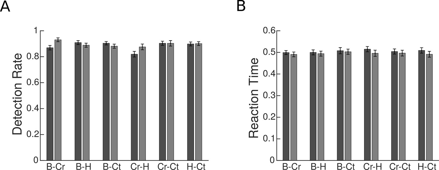
Behavioral performance of the participants during the recording.

B, Cr, H, and Ct represent the Body, Car, House, and Cat categories, respectively. Each x-axis label represents the two conditions with stimuli from the same two categories but with different attentional targets, with the dark gray bar illustrating the results related to the condition in which the first category was attended, and the light gray bar representing the results in the condition in which the second category was attended. For instance, the B-Cr bars represent the results related to the $B o d y^{a t} C a r$ and $B o d y C a r^{a t}$ conditions, respectively. Error bars represent standard errors of the mean. N=15 human participants. (A) Average detection rate for each category pair. (B) Average reaction time for each category pair.

Figure 2

Download asset Open asset

Response vectors related to $x$ and $y$ stimuli in isolated and paired conditions.

(A) Example illustration of the isolated and paired responses in three-dimensional space. $V_{x^{a t}}$ and $V_{y^{a t}}$ denote the response vectors related to isolated $x$ and isolated $y$ conditions and $V_{x^{a t} y}$ illustrates the response in the paired condition with attention directed to stimulus $x$ . The paired response is projected on the plane defined by the two isolated responses $V_{x^{a t}}$ and $V_{y^{a t}}$ . This projection is illustrated by $P_{x^{a t} y}$ . (B) Two-dimensional illustration of the plane defined by the two isolated response vectors $V_{x^{a t}}$ and $V_{y^{a t}}$ , along with the paired response vectors $V_{x^{a t}}$ and $V_{y^{a t}}$ and $P_{x^{a t} y}$ as the projection of the paired response, $V_{x^{a t} y}$ , on the plane. We calculated the weight of the two isolated responses in the paired response using multiple regression, with the weights of $V_{x^{a t}}$ and $V_{y^{a t}}$ shown as $a_{1}$ and $a_{2}$ , respectively.

Figure 3

Download asset Open asset

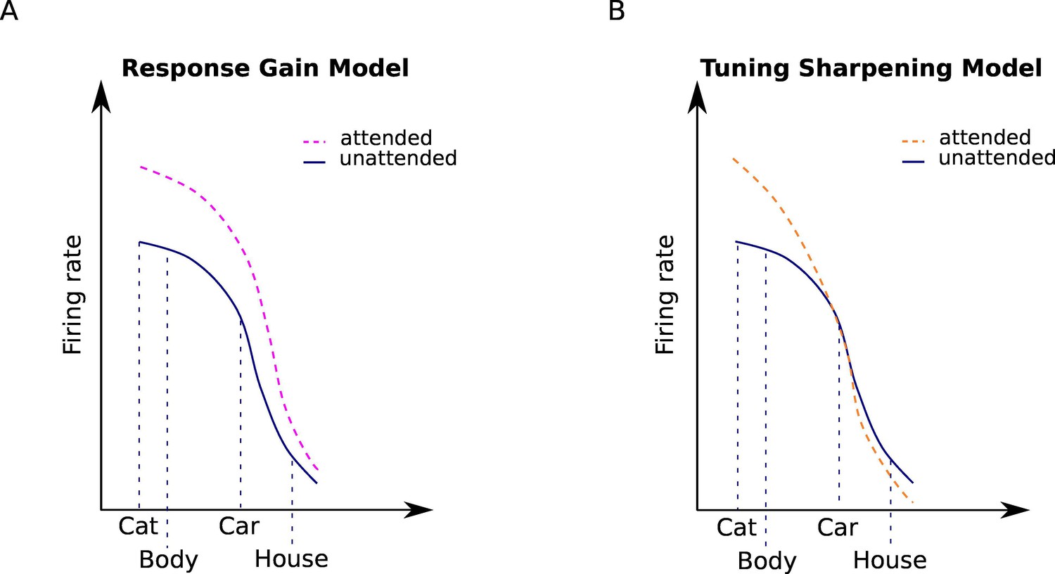
Attentional modulation by the response gain and tuning sharpening models.

We illustrate the models here for the example of a neuron with high selectivity for cat stimuli. Solid curves denote the response to unattended stimuli and dashed curves denote the response to attended stimuli. (A) According to the response gain model, the response of the neuron to attended stimuli is scaled by a constant attention factor. Therefore, the response of the cat-selective neuron to an attended stimulus is enhanced to the same degree for all stimuli. (B) According to the tuning sharpening model, the response modulation by attention depends on the neuron’s tuning for the attended stimulus. Therefore, for optimal and near-optimal stimuli such as cat and body stimuli the response is highly increased, while for non-optimal stimuli such as houses, the response is suppressed.

Figure 4 with 4 supplements

Download asset Open asset

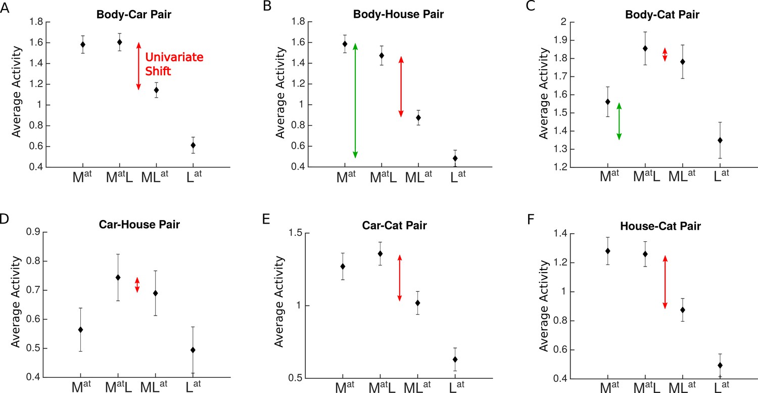
Average voxel response in the extastriate body area (EBA) for each pair of stimulus categories.

The x-axis labels represent the four conditions related to each category pair, $M^{a t}$ , $M^{a t} L$ , $M L^{a t}$ , $L^{a t}$ , with $M$ and $L$ denoting the presence of the more preferred and the less preferred category and the superscript $a t$ denoting the attended category. For instance, $M^{a t}$ refers to the condition in which the more preferred stimulus was presented in isolation (and automatically attended), and $M L^{a t}$ refers to the paired condition in which the less preferred stimulus was attended to. Red arrows in each panel illustrate the observed change in response (univariate shift) caused by the shift of attention from the more preferred to the less preferred stimulus. Green arrows in panels B and C illustrate the difference in the response to isolated stimuli. Error bars represent standard errors of the mean. N=17 human participants.

Figure 4—figure supplement 1

Download asset Open asset

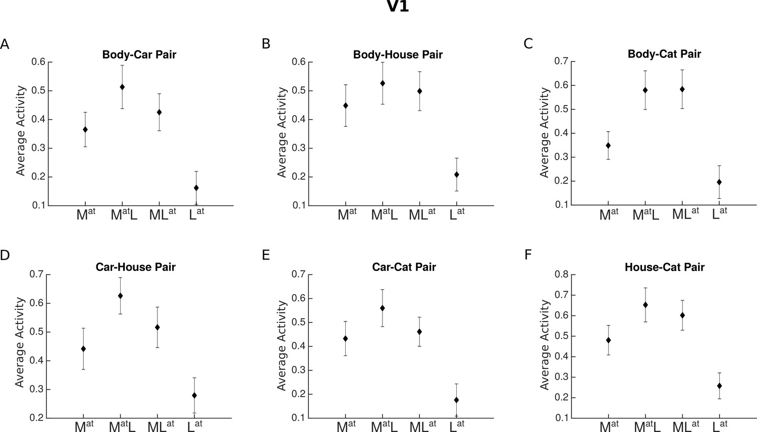
Average voxel response in the primary visual cortex (V1) for each pair of stimulus categories.

The x-axis labels represent the four conditions related to each category pair, $M^{a t}$ , $M^{a t} L$ , $M L^{a t}$ , $L^{a t}$ , with $M$ , and $L$ denoting the presence of the more preferred and the less preferred category and the superscript $a t$ denoting the attended category. For instance, $M^{a t}$ refers to the condition in which the more preferred stimulus was presented in isolation (and automatically attended), and $M L^{a t}$ refers to the paired condition in which the less preferred stimulus was attended to.

Figure 4—figure supplement 2

Download asset Open asset

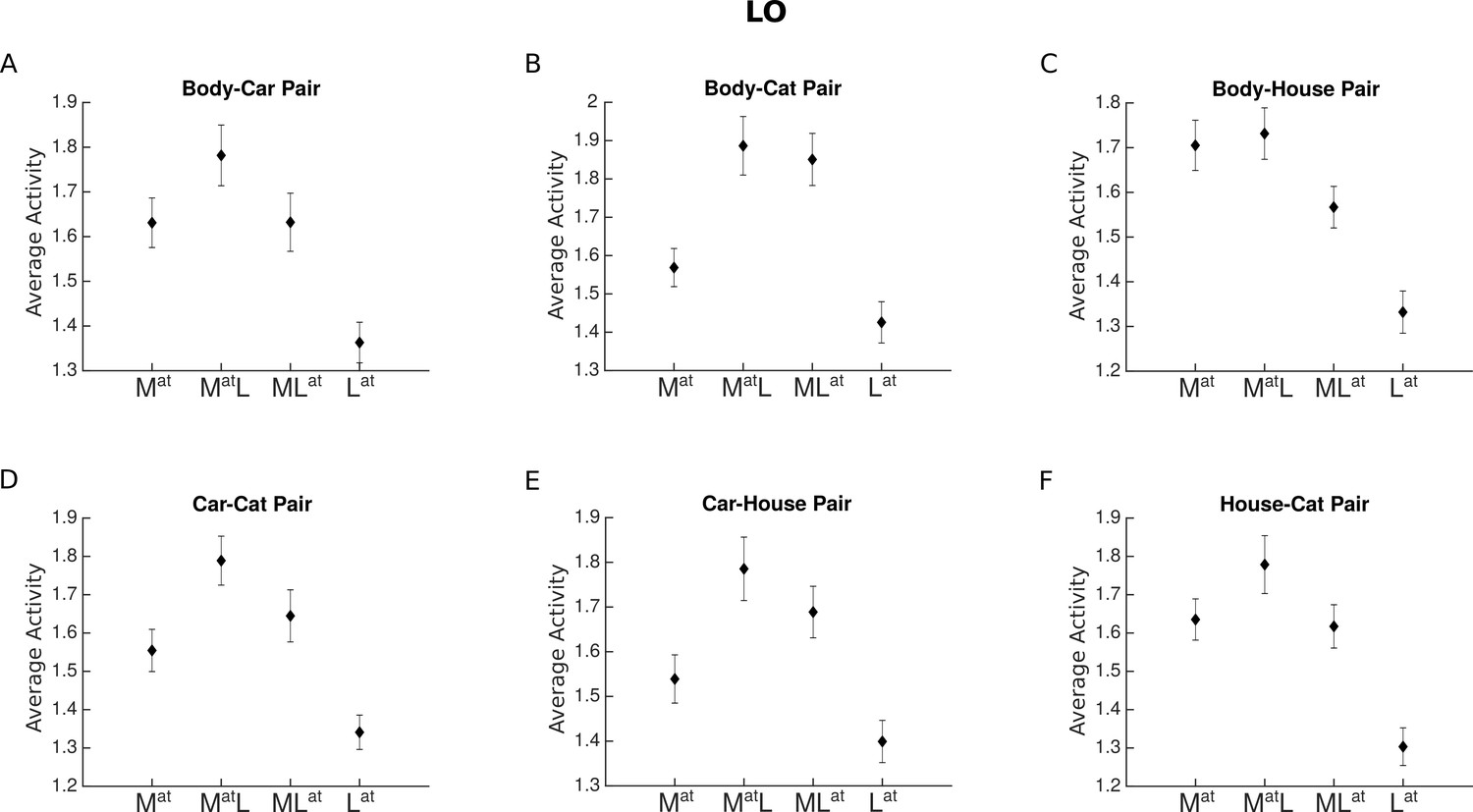
Average voxel response in the lateral occipital cortex (LO) for each pair of stimulus categories.

The x-axis labels represent the four conditions related to each category pair, $M^{a t}$ , $M^{a t} L$ , $M L^{a t}$ , $L^{a t}$ , with $M$ , and $L$ denoting the presence of the more preferred and the less preferred category and the superscript $a t$ denoting the attended category.

Figure 4—figure supplement 3

Download asset Open asset

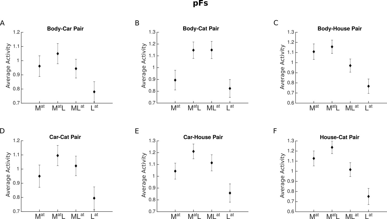
Average voxel response in the posterior fusiform gyrus (pFs) for each pair of stimulus categories.

The x-axis labels represent the four conditions related to each category pair, $M^{a t}$ , $M^{a t} L$ , $M L^{a t}$ , $L^{a t}$ , with $M$ , and $L$ denoting the presence of the more preferred and the less preferred category and the superscript $a t$ denoting the attended category.

Figure 4—figure supplement 4

Download asset Open asset

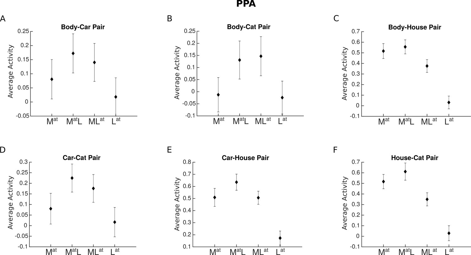
Average voxel response in the parahippocampal place area (PPA) for each pair of stimulus categories.

The x-axis labels represent the four conditions related to each category pair, $M^{a t}$ , $M^{a t} L$ , $M L^{a t}$ , $L^{a t}$ , with $M$ , and $L$ denoting the presence of the more preferred and the less preferred category and the superscript $a t$ denoting the attended category.

Figure 5

Download asset Open asset

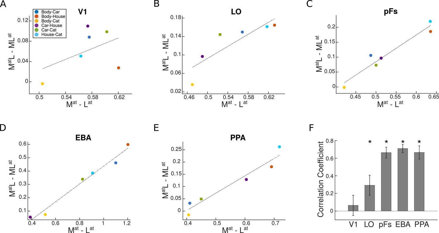
Univariate shift versus category distance in each region of interest (ROI).

(**A–E**) The value of univariate shift versus category distance. $M^{a t} L$ and $M L^{a t}$ denote the two paired conditions with attention directed to the more preferred (M) or less preferred (L) stimulus, respectively. $M^{a t}$ and $L^{a t}$ represent the isolated conditions, respectively, with the more preferred or the less preferred stimulus presented in isolation. The blue, red, yellow, purple, green, and sky blue circles in each panel represent the values related to the Body-Car, Body-House, Body-Cat, Car-House, Car-Cat, and House-Cat pairs, respectively. The correlation coefficients in each ROI were calculated for single participants and the lines in the average plots are only shown for illustration purposes. (F) Correlation coefficient for the correlation between the univariate shift and category distance in each ROI. Asterisks indicate that the correlation coefficients are significantly positive ( $p < 0.05$ ). Error bars represent standard errors of the mean. N=17 human participants.

Figure 6 with 1 supplement

Download asset Open asset

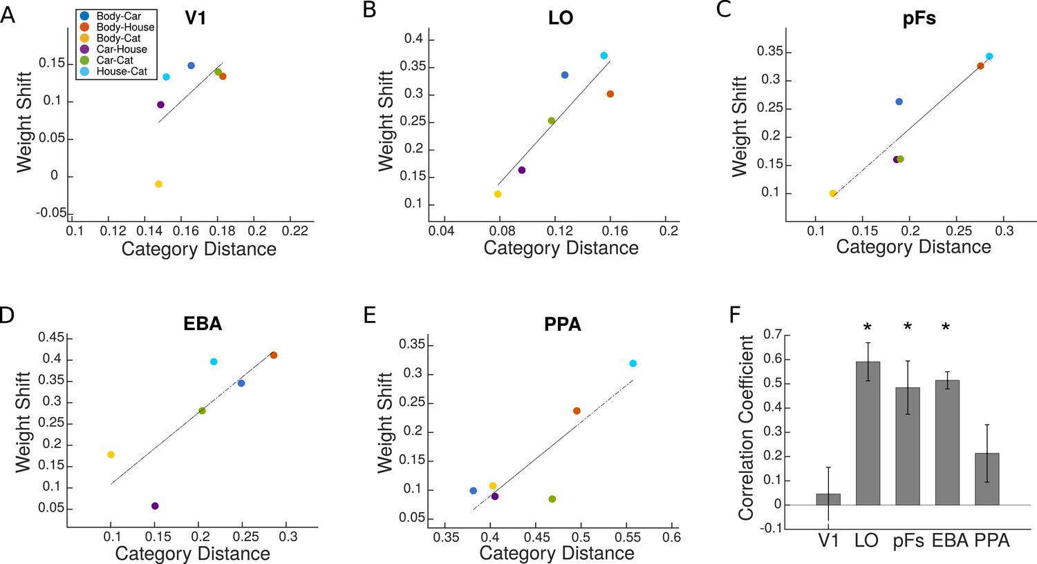
Weight shift versus category distance in each region of interest (ROI).

(**A–E**) Attentional weight shift versus category distance. The blue, red, yellow, purple, green, and sky blue circles in each panel represent the values related to the Body-Car, Body-House, Body-Cat, Car-House, Car-Cat, and House-Cat pairs, respectively. We calculated the correlation coefficients for single participants and the lines in these average plots are only for illustration purposes. (F) Correlation coefficient for the correlation between attentional weight shift and category distance in each ROI. Asterisks indicate that the correlations are significantly positive ( $p < 0.05$ ). Error bars represent standard errors of the mean. N=17 human participants.

Figure 6—figure supplement 1

Download asset Open asset

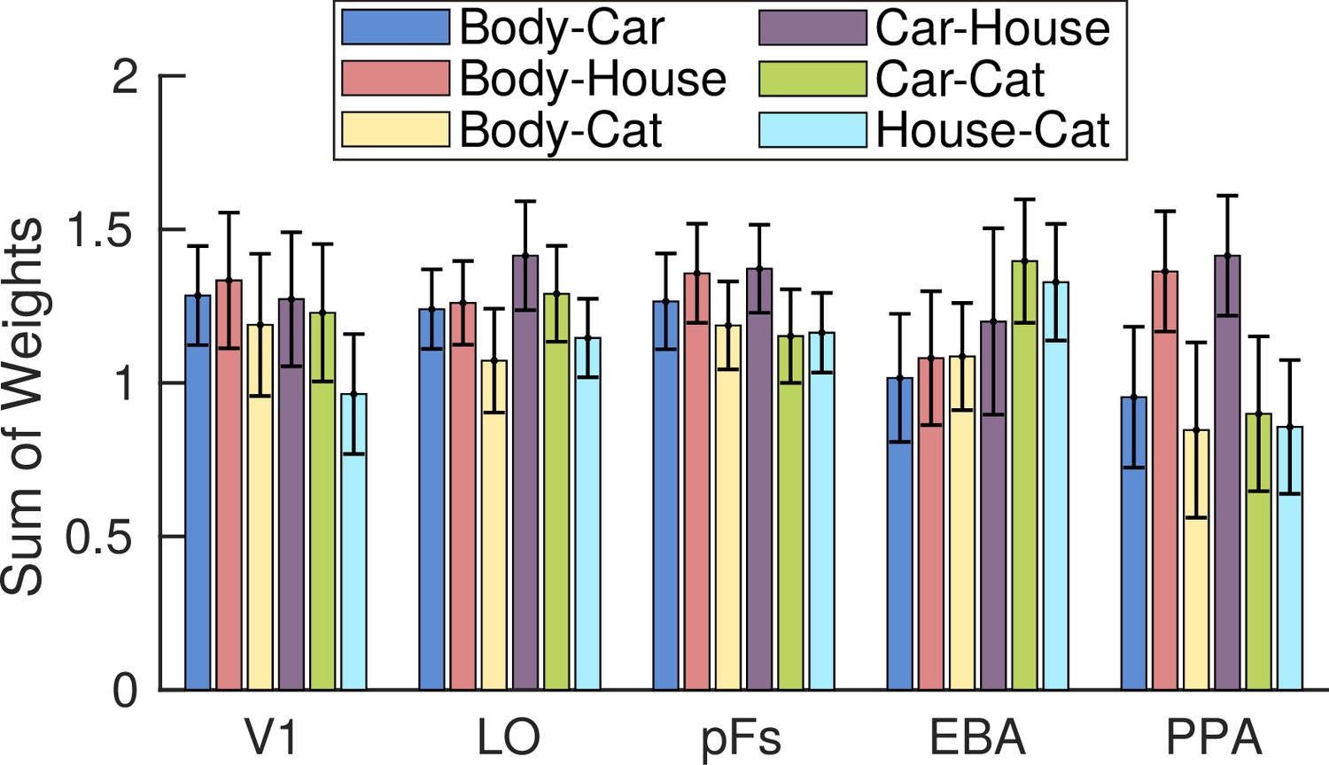
Sum of weights in the multivariate analysis for each category pair in each region of interest (ROI), averaged across conditions with attention directed to each of the two categories of a pair and across participants.

For instance, the blue Body-Car bars represent the average results related to the $B o d y^{a t} C a r$ and $B o d y C a r^{a t}$ conditions, averaged across participants. Error bars represent standard errors of the mean. N=17 human participants.

Figure 7

Download asset Open asset

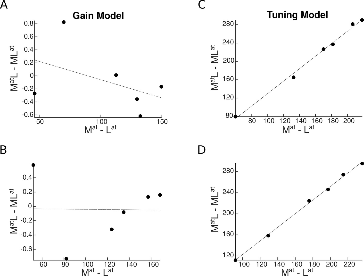
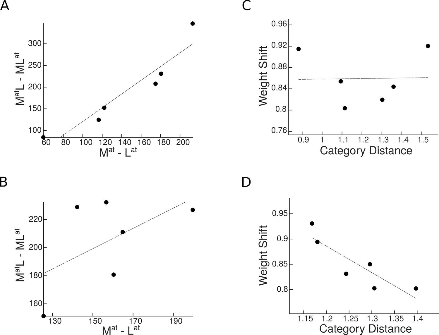
Univariate shift as a function of category distance, as predicted by the two attentional mechanisms.

$M^{a t} L$ and $M L^{a t}$ denote the two paired conditions with attention directed to the more preferred ( $M$ ) or the less preferred ( $L$ ) stimulus, respectively. $M^{a t}$ and $L^{a t}$ represent the isolated conditions, respectively with the $M$ or the $L$ stimulus presented in isolation. Top panels represent predictions in a region with a strong preference for a specific category, and bottom panels illustrate predictions in an object-selective region. Each circle represents a pair of categories. (**A–B**) Predicted univariate shift based on the response gain model in a region with a strong preference for a specific category (A) and in an object-selective region (B). (**C–D**) Predicted univariate shift based on the tuning model in a region with strong preference for a specific category (C) and in an object-selective region (D).

Figure 8

Download asset Open asset

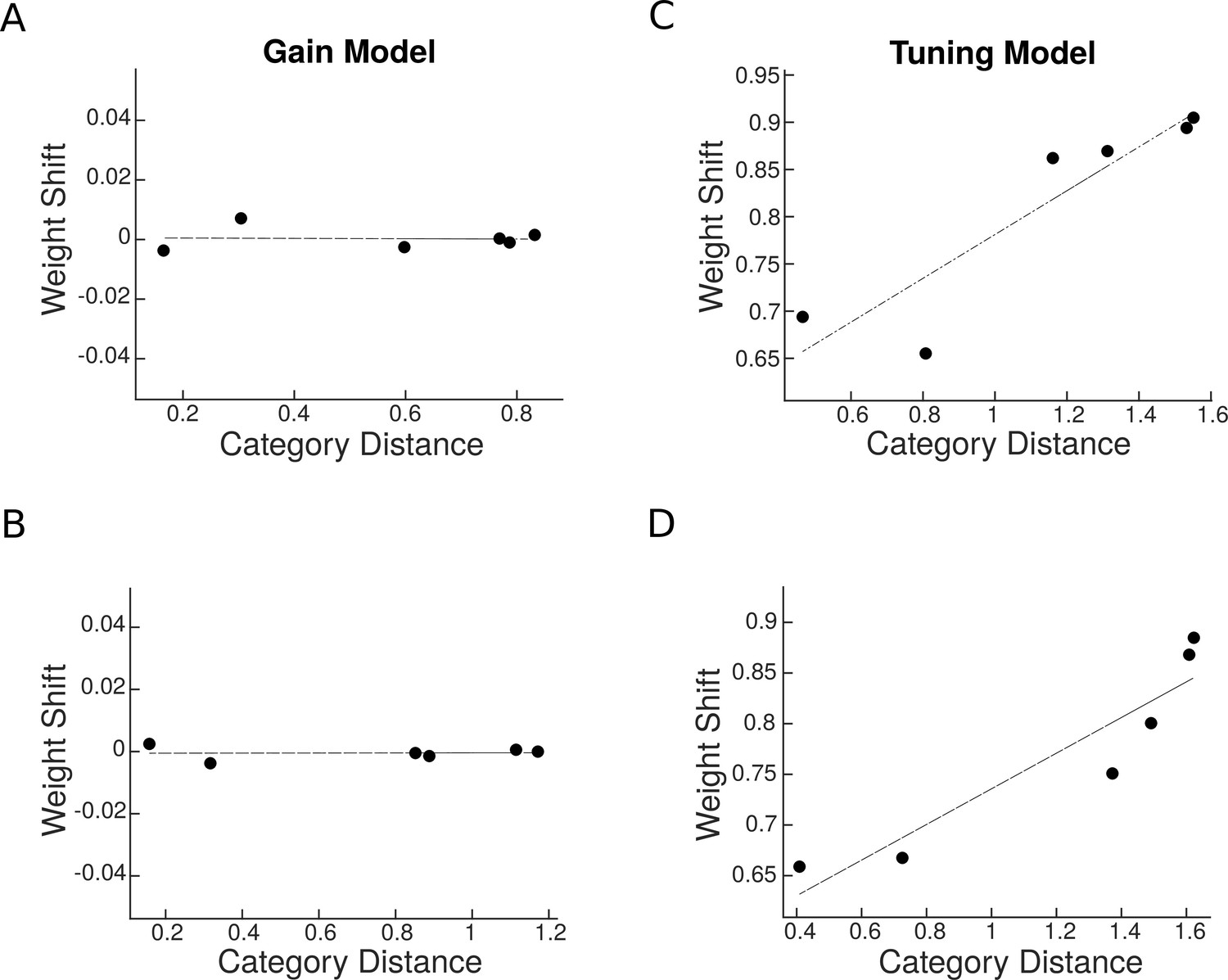
Predicted weight shift as a function of category distance.

Weight shift for each pair is calculated using Equation 5. Category distance represents the difference in multi-voxel representation between responses to the two isolated stimuli, calculated by Equation 3. Top panels are related to predictions in a region with a strong preference for a specific category and the bottom panels illustrate predictions in an object-selective region. (**A–B**) Weight shift predicted by the response gain model in a region with a strong preference for a specific category (A) and in an object-selective region (B). (**C–D**) Weight shift predicted by the tuning model in a region with strong preference for a specific category (C) and in an object-selective region (D).

Appendix 1—figure 1

Download asset Open asset

Based on the labeled line model, attention enhances the response of a neuron only when the attended stimulus is the neuron’s preferred stimulus.

We illustrate the models here for the example of a neuron with high selectivity for cat stimuli. Solid curves denote the response to unattended stimuli and dashed curves denote the response to attended stimuli.

Appendix 1—figure 2

Download asset Open asset

Simulation results for the labeled line model.

(**A–B**) Predicted univariate shift based on the labeled line model in a region with a strong preference for a specific category (A) and in an object-selective region (B). (**C–D**) Weight shift predicted by the labeled line model in a region with a strong preference for a specific category (C) and in an object-selective region (D).

Author response image 1

Download asset Open asset

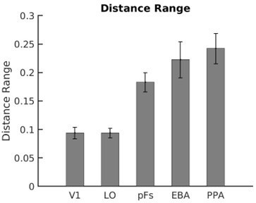
Range of category distance in each ROI averaged across participants.

Author response image 2

Download asset Open asset

Univariate shift versus category distance including single-subject data points in all ROIs.

Author response image 3

Download asset Open asset

Weight shift versus category distance including single-subject data points in all ROIs.

Tables

Appendix 1—table 1

Percentage of voxels in each regions of interest (ROI) most responsive to each of the four stimulus categories, averaged across participants.

Preferred Category	V1	LO	pFs	EBA	PPA
Body	21%	31%	21%	70%	10%
Car	19%	18%	17%	4%	12%
House	33%	32%	40%	3%	68%
Cat	27%	19%	22%	23%	10%

Appendix 1—table 2

Average voxel response (general linear model, GLM coefficients) to each category in each region of interest (ROI), averaged across participants.

Stimulus Category	V1	LO	pFs	EBA	PPA
Body	0.28	1.59	0.88	1.62	0.001
Car	0.28	1.43	0.88	0.60	0.12
House	0.47	1.51	1.03	0.48	0.55
Cat	0.35	1.49	0.89	1.32	–0.02

Appendix 1—table 3

Single-subject correlation coefficients for the correlation between the univariate shift and category distance in all regions of interest (ROIs).

V1	LO	pFs	EBA	PPA
–0.60	0.67	–0.073	0.72	0.18
0.16	0.38	0.015	0.64	0.46
–0.53	0.52	0.89	0.60	0.42
–0.062	0.78	0.93	0.87	0.69
–0.098	0.072	1.0	0.72	0.96
0.63	0.93	0.88	0.94	0.58
–0.31	0.52	–0.11	0.88	0.89
0.29	0.18	0.62	0.67	0.63
–0.49	0.094	0.63	0.81	0.80
0.21	0.57	0.31	0.81	0.87
–0.015	–0.57	0.79	0.35	0.69
0.35	0.79	0.90	0.90	0.88
–0.47	0.058	–0.050	0.93	–0.24
–0.047	–0.21	0.91	0.28	0.86
0.66	0.70	0.91	0.64	0.45
–0.74	0.54	0.24	0.60	–0.31
–0.095	0.73	0.89	0.64	0.95

Appendix 1—table 4

Weights of each stimulus for each category pair in each region of interest (ROI), averaged across participants.

Pair	Attended Stimulus	V1	LO	pFs	EBA	PPA
Body-Car	Body	$0.54 \times R_{B^{a t}} + 0.53 \times R_{C r^{a t}}$	$0.79 \times R_{B^{a t}} + 0.31 \times R_{C r^{a t}}$	$0.68 \times R_{B^{a} t} + 0.42 \times R_{C r^{a t}}$	$0.93 \times R_{B^{a t}} + 0.15 \times R_{C r^{a t}}$	$0.41 \times R_{B^{a t}} + 0.42 \times R_{C r^{a t}}$
Body-Car	Car	$0.40 \times R_{B^{a t}} + 0.70 \times R_{C r^{a t}}$	$0.43 \times R_{B^{a t}} + 0.68 \times R_{C r^{a t}}$	$0.39 \times R_{B^{a t}} + 0.70 \times R_{C r^{a t}}$	$0.53 \times R_{B^{a t}} + 0.46 \times R_{C r^{a t}}$	$0.35 \times R_{B^{a t}} + 0.54 \times R_{C r^{a t}}$
Body-House	Body	$0.43 \times R_{B^{a t}} + 0.65 \times R_{H^{a t}}$	$0.65 \times R_{B^{a t}} + 0.45 \times R_{H^{a t}}$	$0.65 \times R_{B^{a t}} + 0.47 \times R_{H^{a t}}$	$0.84 \times R_{B^{a t}} + 0.21 \times R_{H^{a t}}$	$0.42 \times R_{B^{a t}} + 0.61 \times R_{H^{a t}}$
Body-House	House	$0.27 \times R_{B^{a t}} + 0.78 \times R_{H^{a t}}$	$0.3 \times R_{B^{a t}} + 0.74 \times R_{H^{a t}}$	$0.27 \times R_{B^{a t}} + 0.81 \times R_{H^{a t}}$	$0.37 \times R_{B^{a t}} + 0.57 \times R_{H^{a t}}$	$0.18 \times R_{B^{a t}} + 0.86 \times R_{H^{a t}}$
Body-Cat	Body	$0.63 \times R_{B^{a t}} + 0.55 \times R_{C t^{a t}}$	$0.86 \times R_{B^{a t}} + 0.35 \times R_{C t^{a t}}$	$0.81 \times R_{B^{a t}} + 0.45 \times R_{C t^{a t}}$	$0.90 \times R_{B^{a t}} + 0.30 \times R_{C t^{a t}}$	$0.61 \times R_{B^{a t}} + 0.32 \times R_{C t^{a t}}$
Body-Cat	Cat	$0.59 \times R_{B^{a t}} + 0.55 \times R_{C t^{a t}}$	$0.69 \times R_{B^{a t}} + 0.48 \times R_{C t^{a t}}$	$0.67 \times R_{B^{a t}} + 0.55 \times R_{C t^{a t}}$	$0.67 \times R_{B^{a t}} + 0.48 \times R_{C t^{a t}}$	$0.55 \times R_{B^{a t}} + 0.37 \times R_{C t^{a t}}$
Car-House	Car	$0.42 \times R_{C r^{a t}} + 0.65 \times R_{H^{a t}}$	$0.44 \times R_{C r^{a t}} + 0.70 \times R_{H^{a t}}$	$0.55 \times R_{C r^{a t}} + 0.60 \times R_{H^{a t}}$	$0.56 \times R_{C r^{a t}} + 0.59 \times R_{H^{a t}}$	$0.35 \times R_{C r^{a t}} + 0.72 \times R_{H^{a t}}$
Car-House	House	$0.31 \times R_{C r^{a t}} + 0.73 \times R_{H^{a t}}$	$0.25 \times R_{C r^{a t}} + 0.85 \times R_{H^{a t}}$	$0.36 \times R_{C r^{a t}} + 0.78 \times R_{H^{a t}}$	$0.46 \times R_{C r^{a t}} + 0.65 \times R_{H^{a t}}$	$0.27 \times R_{C r^{a t}} + 0.93 \times R_{H^{a t}}$
Car-Cat	Car	$0.59 \times R_{C r^{a t}} + 0.52 \times R_{C t^{a t}}$	$0.68 \times R_{C r^{a t}} + 0.44 \times R_{C t^{a t}}$	$0.74 \times R_{C r^{a t}} + 0.40 \times R_{C t^{a t}}$	$0.47 \times R_{C r^{a t}} + 0.54 \times R_{C t^{a t}}$	$0.53 \times R_{C r^{a t}} + 0.40 \times R_{C t^{a t}}$
Car-Cat	Cat	$0.45 \times R_{C r^{a t}} + 0.70 \times R_{C t^{a t}}$	$0.41 \times R_{C r^{a t}} + 0.75 \times R_{C t^{a t}}$	$0.55 \times R_{C r^{a t}} + 0.60 \times R_{C t^{a t}}$	$0.23 \times R_{C r^{a t}} + 0.92 \times R_{C t^{a t}}$	$0.46 \times R_{C r^{a t}} + 0.46 \times R_{C t^{a t}}$
House-Cat	House	$0.76 \times R_{H^{a t}} + 0.32 \times R_{C t^{a t}}$	$0.87 \times R_{H^{a t}} + 0.24 \times R_{C t^{a t}}$	$0.91 \times R_{H^{a t}} + 0.23 \times R_{C t^{a t}}$	$0.56 \times R_{H^{a t}} + 0.44 \times R_{C t^{a t}}$	$0.99 \times R_{H^{a t}} + 0.11 \times R_{C t^{a t}}$
House-Cat	Cat	$0.61 \times R_{H^{a t}} + 0.47 \times R_{C t^{a t}}$	$0.47 \times R_{H^{a t}} + 0.65 \times R_{C t^{a t}}$	$0.53 \times R_{H^{a t}} + 0.62 \times R_{C t^{a t}}$	$0.17 \times R_{H^{a t}} + 0.90 \times R_{C t^{a t}}$	$0.57 \times R_{H^{a t}} + 0.38 \times R_{C t^{a t}}$

Appendix 1—table 5

Single-subject correlation coefficients for the correlation between weight shift and category distance in all regions of interests (ROIs).

V1	LO	pFs	EBA	PPA
–0.36	0.93	–0.25	0.46	0.06
0.31	–0.06	0.16	0.82	–0.25
–0.29	0.35	0.80	0.48	–0.42
–0.038	0.70	0.75	0.57	0.38
0.72	0.60	0.90	0.58	–0.77
0.53	0.69	0.76	0.51	0.59
–0.32	0.90	–0.25	0.29	0.065
0.33	0.22	–0.36	0.24	–0.48
0.52	0.31	0.63	0.54	0.91
0.019	0.96	0.80	0.61	0.71
–0.11	0.87	0.89	0.69	0.51
–0.27	0.94	0.81	0.63	0.50
–0.28	0.28	–0.11	0.49	0.59
0.42	0.11	0.61	0.42	0.59
0.67	0.77	0.78	0.36	0.36
–0.96	0.78	0.48	0.43	–0.24
–0.12	0.69	0.82	0.63	0.56

Additional files

MDAR checklist: https://cdn.elifesciences.org/articles/89836/elife-89836-mdarchecklist1-v1.pdf
Download elife-89836-mdarchecklist1-v1.pdf

Download links

A two-part list of links to download the article, or parts of the article, in various formats.

Downloads (link to download the article as PDF)

Open citations (links to open the citations from this article in various online reference manager services)

Mendeley

Cite this article (links to download the citations from this article in formats compatible with various reference manager tools)

Narges Doostani
Gholam-Ali Hossein-Zadeh
Radoslaw M Cichy
Maryam Vaziri-Pashkam

(2024)

Attention modulates human visual responses to objects by tuning sharpening

eLife 12:RP89836.

https://doi.org/10.7554/eLife.89836.3

Share this article

Cite this article

Stimuli, paradigm, and regions of interest.

Behavioral performance of the participants during the recording.

Response vectors related to x and y stimuli in isolated and paired conditions.

Attentional modulation by the response gain and tuning sharpening models.

Average voxel response in the extastriate body area (EBA) for each pair of stimulus categories.

Average voxel response in the primary visual cortex (V1) for each pair of stimulus categories.

Average voxel response in the lateral occipital cortex (LO) for each pair of stimulus categories.

Average voxel response in the posterior fusiform gyrus (pFs) for each pair of stimulus categories.

Average voxel response in the parahippocampal place area (PPA) for each pair of stimulus categories.

Univariate shift versus category distance in each region of interest (ROI).

Weight shift versus category distance in each region of interest (ROI).

Sum of weights in the multivariate analysis for each category pair in each region of interest (ROI), averaged across conditions with attention directed to each of the two categories of a pair and across participants.

Univariate shift as a function of category distance, as predicted by the two attentional mechanisms.

Predicted weight shift as a function of category distance.

Based on the labeled line model, attention enhances the response of a neuron only when the attended stimulus is the neuron’s preferred stimulus.

Simulation results for the labeled line model.

Range of category distance in each ROI averaged across participants.

Univariate shift versus category distance including single-subject data points in all ROIs.

Weight shift versus category distance including single-subject data points in all ROIs.

Percentage of voxels in each regions of interest (ROI) most responsive to each of the four stimulus categories, averaged across participants.

Average voxel response (general linear model, GLM coefficients) to each category in each region of interest (ROI), averaged across participants.

Single-subject correlation coefficients for the correlation between the univariate shift and category distance in all regions of interest (ROIs).

Weights of each stimulus for each category pair in each region of interest (ROI), averaged across participants.

Single-subject correlation coefficients for the correlation between weight shift and category distance in all regions of interests (ROIs).

MDAR checklist

Downloads (link to download the article as PDF)

Open citations (links to open the citations from this article in various online reference manager services)

Cite this article (links to download the citations from this article in formats compatible with various reference manager tools)

Response vectors related to $x$ and $y$ stimuli in isolated and paired conditions.