A neuromorphic model of active vision shows how spatiotemporal encoding in lobula neurons can aid pattern recognition in bees
- Department of Computer Science, University of Sheffield, United Kingdom
- School of Biosciences, University of Sheffield, United Kingdom
- Neuroscience Institute, University of Sheffield, United Kingdom
- School of Biological and Behavioural Sciences, Queen Mary University of London, United Kingdom
- Drone Development Lab, Ben Thorns Ltd, United Kingdom
- School of Natural Sciences, Macquarie University, Australia
- Opteran Technologies Ltd, United Kingdom
Figures
Figure 1

Neural network of active vision inspired by neurobiology and flight dynamics of bees.
(A) The right side displays the front view of the bumblebee head showing the component eye and antenna. Left-hand side presents a schematic view of the bee’s brain regions. Part of neural pathways from the retina to the mushroom bodies is also represented. Labels: AL, antennal lobe; LH, lateral horn; CC, central complex; La, lamina; Me, medulla; Lo, lobula; MB, mushroom body. Figure was designed by Alice Bridges. (B) A representation of the modelled bee’s scanning behaviour of a flower demonstrating how a sequence of patches project to the simulated bee’s eye with lateral movement from left to right. Below are five image patches sampled by the simulated bee. (C) Representation of the neural network model of active vision inspired by micromorphology of the bee brain that underlie learning, memory, and experience-dependent control of behaviour. The photoreceptors located in the eye are excited by the input pattern. The activities of photoreceptors change the membrane potential of a neuron in the next layer, lamina. The lamina neurons send signals (through W connectivity matrix) to the medulla neurons to generate spikes in this layer. Each wide-field lobula neuron integrates the synaptic output of five small-field medulla neurons. The lobula neurons are laterally inhibited by local lobula interconnections (via Q connectivity matrix). Lobula neurons project their axons into the mushroom body, forming connections with Kenyon cells (KCs) through a randomly weighted connectivity matrix, S. The KCs all connect to a single mushroom body output neuron (MBON) through random synaptic connections D. A single reinforcement neuron (yellow neuron) modulates the synaptic weights between KCs and MBON by simulating the release of octopamine or dopamine when presented with specific visual stimuli (see Methods). (D) A temporal coding model that is proposed as the connectivity between medulla and lobula neurons. Each matrix shows the inhibitory (blue) and excitatory (red) connectivity between lamina neurons to a medulla neuron at a given time delay. In this model, the five small-field medulla neurons that are activated by the locally visual input, at different times of scanning, send their activities to a wide-field lobula neuron with a synaptic delay such that the lobula neuron receives all medulla input signals at the same instance (i.e. in the presented simulation the lobula neuron is maximally activated by the black vertical bar passing across the visual field from the left to right. Each underlying medulla neuron encodes the vertical bar in a different location of the visual field).
Figure 2 with 1 supplement
Neural responses of the simulated bee model to visual patterns.
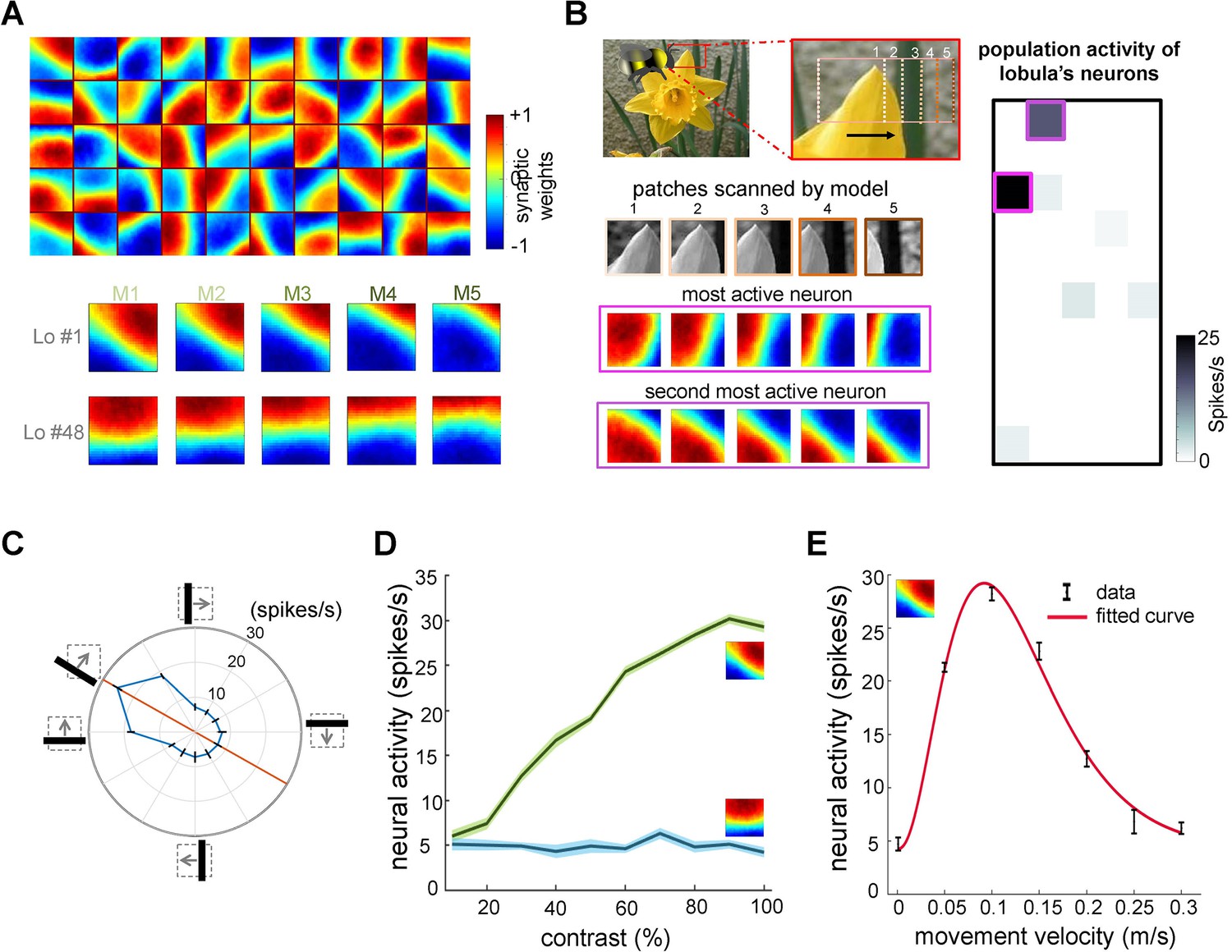
(A) Top: each square in the matrix corresponds to a single time slice of the obtained spatiotemporal receptive field of a lobula neuron (5 × 10 lobula neurons) that emerged from non-associative learning in the visual lobes after exposing the model to images of flowers and nature scenes (see Video 3). Bottom: spatiotemporal receptive field of two example lobula neurons are visualised in the five-time delay slices of the matrices of synaptic connectivity between lamina and five medulla neurons (see Figure 1D). The lobula neuron integrates signals from these medulla neurons at each of five time periods as the simulated bees scan a pattern (time goes from left to right). Blue and red cells show inhibitory and excitatory synaptic connectivity, respectively. The first example lobula neuron (#1) encodes the 150° angled bar moving from lower left to the upper right of the visual field. The second example lobula neuron (#48) encodes the movement of the horizontal bar moving up in the visual field. (B) An example of an image sequence projected to the simulated bee’ eye with lateral movement from left to right. Below shows the five images patched sampled by the simulated bee. The right side presents the firing rate of all lobula neurons responding to the image sequence. The spatiotemporal receptive field of two highest active neurons to the image sequence are highlighted in purple. (C) The polar plot shows the average orientation selectivity of one example lobula neuron (#1) to differently angled bars moving across the visual field in a direction orthogonal to their axis (average of 50 simulations). This neuron is most sensitive to movement when the bar orientation is at 150°. (D) The spiking response of the lobula neuron to the preferred orientation raised as the contrast was increased, whereas the response of the lobula neuron to a non-preferred orientation is maintained irrespective of contrast. (E) The average velocity–sensitivity curve (± SEM) of the orientation-sensitive lobula neuron (#1) is obtained from the responses of the lobula neuron to optimal (angle of maximum sensitivity) moving stimuli presented to the model at different velocities. The red line shows the Gamma function fitted to the data.
Figure 2—figure supplement 1
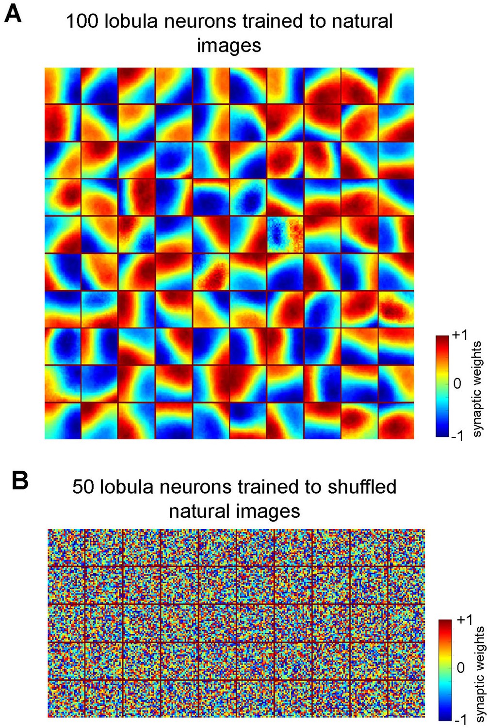
Emergence of receptive fields in Lobula neurons requires structured natural inputs.
(A) Spatiotemporal receptive fields of lobula neurons emerging from non-associative learning when the number of lobula neurons is set to 100 (see Video 2).The details follow those described in Figure 2A. (B) Spatiotemporal receptive fields of 50 lobula neurons trained with shuffled natural images. The neurons fail to develop meaningful connections, resulting in random synaptic weight distributions, indicating that spatial coherence in training images is essential for efficient feature extraction.
Figure 3
Effect of non-associative learning on lobula neuron activity and response sparseness.
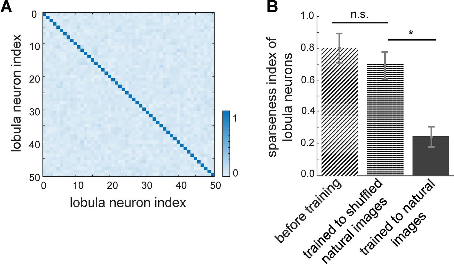
(A) Correlation matrix of lobula neuron responses after training with natural images. The near-diagonal structure indicates that neurons develop distinct and strongly uncorrelated responses, suggesting an efficient, decorrelated representation of visual input. (B) Sparseness index of lobula neurons before and after training with different image sets. Before training, neural responses are broadly distributed. Training with shuffled natural images does not change the sparseness of lobula population, whereas training with natural images significantly increases response sparseness, indicating that exposure to structured visual inputs enhances efficient coding. Error bars represent SEM. Asterisks (*) indicate p-values <0.05, while ‘n.s.’ denotes non-significant results.
Figure 4
Simulated bees’ performance in a pattern recognition task using different scanning strategies.
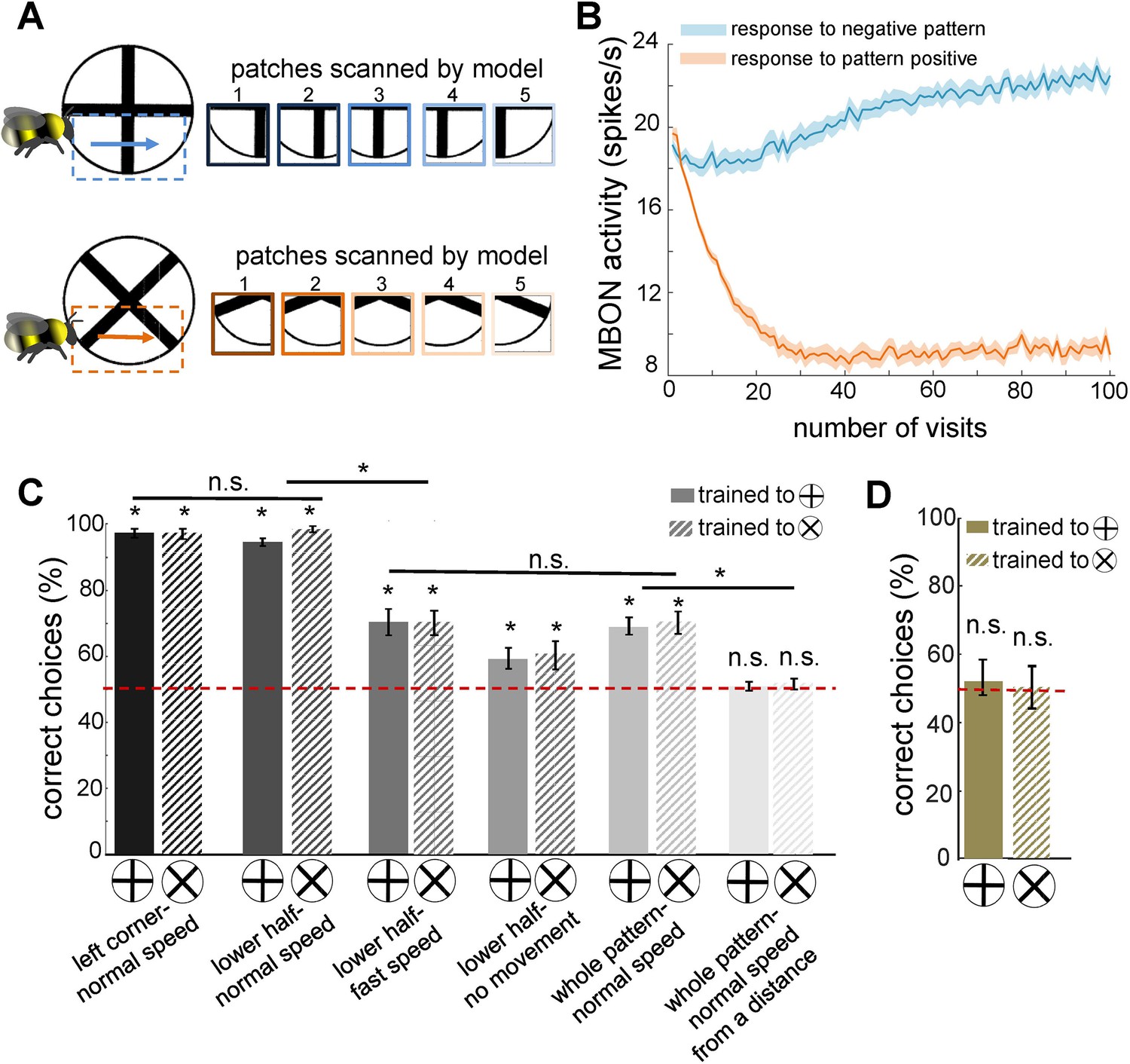
Twenty simulated bees, with random initial neuronal connectivity in mushroom bodies (see Methods) and a fixed connectivity in the visual lobe that were shaped from the non-associative learning, were trained to discriminate a plus from a multiplication symbol (100 random training exposures per pattern). The simulated bees scanned different regions of the patterns at different speeds. (A) Top and below panels show the five image patches sampled from the plus and multiplication symbols by simulated bees, respectively. It is assumed that the simulated bees scanned the lower half of the patterns with lateral movement from left to right with normal speed (0.1 m/s). (B) The plot shows the average responses of the mushroom body output neuron (MBON) to rewarding multiplication and punishing plus patterns during training procedure (multiplication symbol rewarding, producing an Octopamine release by the reinforcement neuron, and the plus symbol inducing a Dopamine release). This shows how the response of the MBON to the rewarding plus was decreased while its response to the punishing multiplication pattern was increased during the training. The MBON equally responded to both multiplication and plus before the training (at number of visits = 0). (C) The performance of the simulated bees in discriminating the right-angled plus and a 45° rotated version of the same cross (i.e. multiplication symbol) (MaBouDi et al., 2025; Srinivasan, 1994), when the stimulated bees scanned different regions of the pattern (left corner, lower half, whole pattern) at different speeds: no speed 0.0 m/s (i.e. all medulla to lobula temporal slices observed the same visual input), normal speed at 0.1 m/s and fast speed at 0.3 m/s, and from a simulated distance of 2 cm from stimuli (default) and 10 cm (distal view). The optimal model parameters were for the stimulated bees at the default distance when only a local region of the pattern (bottom half or lower left quadrant) was scanned at a normal speed. (D) Mean performance (± SEM) of two groups of simulated bees in discriminating the plus from multiplication patterns when their inhibitory connectivity between lobula neurons were not modified by non-associative learning rules. Asterisks (*) indicate p-values < 0.05, while ‘n.s.’ denotes non-significant results.
Figure 5
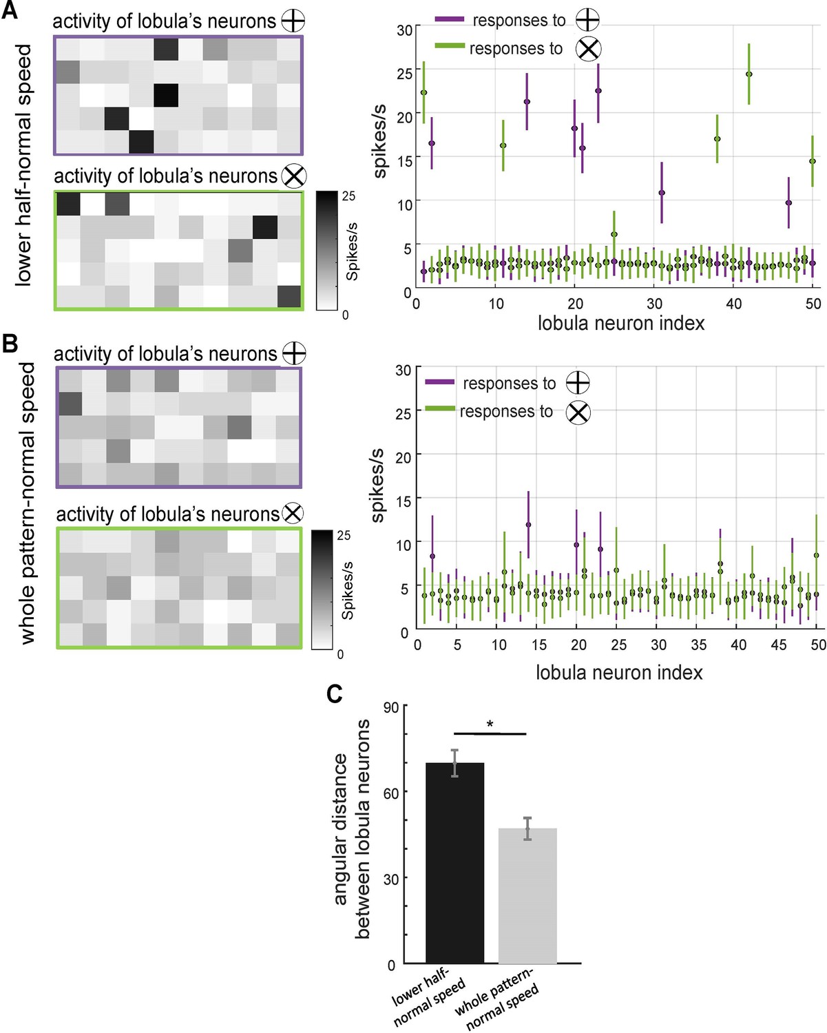
The effect of scanning behaviour on the spatiotemporal encoding of visual patterns in lobula neurons responses.
(A, B) Neural responses of simulated lobula neurons to different scanning conditions. Left panels: heatmaps showing the spiking activity of 50 lobula neurons in response to visual patterns when scanning either the lower half of the pattern at normal speed (A) or the whole pattern at normal speed (B). Right panels: the mean and standard deviation of the spike rate responses of individual lobula neurons to two distinct visual patterns (plus and multiplication), with colour-coded responses (purple for ⊕, green for ⊗). Scanning behaviour significantly alters the neural responses, with distinct sets of neurons preferentially responding to each stimulus. (C) Mean angular distance between lobula neuron responses for different scanning conditions. Lower half-normal speed scanning results in greater separation between neural representations, suggesting that scanning of local region enhances feature selectivity. Error bars represent SEM. Asterisks (*) indicate p-values <0.05, while ‘n.s.’ denotes non-significant results.
Figure 6

Proposed neural network performance to published bee pattern experiments.
Twenty simulated bees, with random initial neuronal connectivity in mushroom bodies (see Methods), were trained to discriminate a positive target pattern from a negative distractor pattern (50 training exposures per pattern). The simulated bees’ performances were examined via unrewarded tests, where synaptic weights were not updated (average of 20 simulated pattern pair tests per bee). All simulations were conducted under the assumption that model bees viewed the targets from a distance of 2 cm while flying at a normal speed of 0.1 m/s. During this process, the bees scanned the lower half of the pattern. (A) Mean percentage of correct choices (± SEM) in discriminating bars oriented at 90° to each other, 25.5° angled cross with a 45° rotated version of the same cross, and a pair of mirrored spiral patterns (MaBouDi et al., 2025; Srinivasan, 1994). The simulated bees achieved greater than chance performances. (B) Performance of simulated bees trained with a generalisation protocol (Benard et al., 2006). Trained to 6 pairs of perpendicular oriented gratings (10 exposures per grating). Simulated bees then tested with a novel gating pair, and a single oriented bar pair. The simulated bees performed well in distinguishing between the novel pair of gratings; less well, but still significantly above chance, to the single bars. This indicates that the model can generalise the orientation of the training patterns to distinguish the novel patterns. (C) Mean performance (± SEM) of the simulated bees in discriminating the positive orientation from negative orientation. Additionally, the performance in recognising the positive orientation from the novel pattern, and preference for the negative pattern from a novel pattern. Simulated bees learnt to prefer positive patterns, but also reject negative patterns, in this case preferring novel stimuli. (D) Performance of simulated bees trained to a horizontal and –45° bar in the lower pattern half versus a vertical and +45° bar (Stach et al., 2004). The simulated bees could easily discriminate between the trained bars, and a colour inverted version of the patterns. They performed less well when the bars were replaced with similarly oriented gratings, but still significantly above chance. When tested on the positive pattern vs. a novel pattern with one correctly and one incorrectly oriented bar, the simulated bees chose the positive patterns (fourth and fifth bars), whereas with the negative pattern versus this same novel pattern the simulated bees rejected the negative pattern in preference for the novel pattern with single positive oriented bar (two last bars). (E) The graph shows the mean percentage of correct choices for the 20 simulated bees during a facial recognition task (Dyer et al., 2005). Simulated bees were trained to the positive (rewarded) face image versus a negative (non-rewarded) distractor face. The model bee is able to recognise the target face from distractors after training, and also to recognise the positive face from novel faces even if the novel face is similar to the target face (fourth bar). However, it failed to discriminate between the positive and negative faces rotated by 180°. (F) The model was trained on spatially structured patterns from Stach et al., 2004, requiring recognition of orientation arrangements across four quadrants. Unlike bees, the model failed to discriminate these patterns, highlighting its limitations in integrating local features into a coherent global representation. Asterisks (*) indicate p-values < 0.05, while ‘n.s.’ denotes non-significant results.
Figure 7
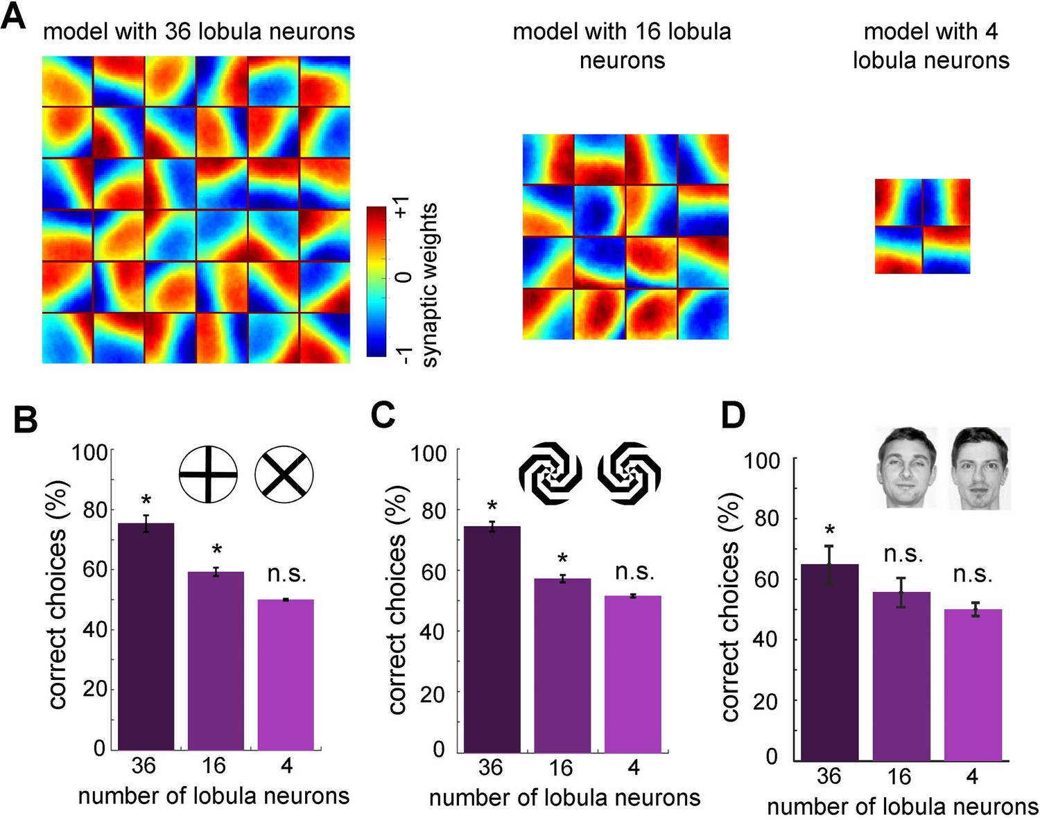
Minimum number of lobula neurons that are necessary for pattern recognition.
(A) Obtained spatiotemporal receptive field of lobula neurons when the number of lobula neurons were set at 36, 16, or 4 during the non-associative learning in the visual lobe (see Figure 5A). This shows the models with lower number of lobula neurons encode less variability of orientations and temporal coding of the visual inputs (see Videos 5 and 6) The average correct choices of the three models with 36, 16, or 4 lobula neurons after training to a pair of plus and multiplication patterns (B), mirrored spiral patterns (C), and human face discrimination (D). The model with 36 lobula neurons still can solve pattern recognition tasks at a level above chance. It indicates that only 36 lobula neurons that provide all inputs to mushroom bodies are sufficient for the simulated bees to be able to discriminate between patterns. Asterisks (*) indicate p-values <0.05, while ‘n.s.’ denotes non-significant results.
Figure 8

The role of lateral inhibitory connections between lobula neurons.
Figure 9

Spike-timing-dependent plasticity (STDP) curves.
(A) Classical spike-timing-dependent plasticity (STDP) curve showing relationship between synaptic weight change and the precise time difference between the Kenyon cells and mushroom body output neuron (MBON) spikes. The synaptic weight can be either depressed or potentiated. (B) STDP curve modulated by octopamine in the insect mushroom body. The Synaptic weights are depressed. The formula of these curves is described in Equations 3 and 4.
Videos
Video 1
Spatiotemporal dynamics of receptive fields in 50 lobula neurons emerging from non-associative learning and active scanning.
Each square in the matrix represents a single time slice of the spatiotemporal receptive field for a lobula neuron (5 × 10 array of neurons). These receptive fields illustrate the connectivity matrix between five medulla neurons and their corresponding lobula neuron, operating under a temporal coding structure. In this framework, each of the five medulla neurons sequentially transfers a portion of the visual input to the lobula neuron through excitatory (red) and inhibitory (blue) synaptic connections. These receptive fields develop within the visual lobes after the model is exposed to natural images, including flowers and scenery. As the simulated bee scans a visual pattern, lobula neurons dynamically integrate inputs from medulla neurons over time, forming a temporally structured neural representation of the visual scene.
Video 2
Spatiotemporal dynamics of receptive fields in 100 lobula neurons emerging from non-associative learning and active scanning.
This follows the same structure as Video 1, depicting the receptive field evolution in a larger population of 100 lobula neurons under the temporal coding framework and non-associative learning.
Video 3
Spatiotemporal dynamics of receptive fields in 36 lobula neurons emerging from non-associative learning and active scanning.
This follows the same structure as Video 1, depicting the receptive field evolution in a larger population of 36 lobula neurons under the temporal coding framework and non-associative learning.
Video 4
Spatiotemporal dynamics of receptive fields in 16 lobula neurons emerging from non-associative learning and active scanning.
This follows the same structure as Video 1, depicting the receptive field evolution in a larger population of 16 lobula neurons under the temporal coding framework and non-associative learning (compare to Videos 1 and 3).
Video 5
Spatiotemporal dynamics of receptive fields in only four lobula neurons emerging from non-associative learning and active scanning.
This follows the same structure as Video 1, depicting the receptive field evolution in a larger population of four lobula neurons under the temporal coding framework and non-associative learning (compare to Videos 1, 3, and 4).
Video 6
Spatiotemporal dynamics of receptive fields in 50 lobula neurons emerging from non-associative learning and active scanning.
This follows the same structure as Video 1, but with fixed lateral inhibitory connectivity between lobula neurons during non-associative learning. The video illustrates how receptive fields evolve under the temporal coding framework, providing a comparison to Video 1, where lateral inhibition was plastic.
Additional files
Download links
A two-part list of links to download the article, or parts of the article, in various formats.
Downloads (link to download the article as PDF)
Open citations (links to open the citations from this article in various online reference manager services)
Cite this article (links to download the citations from this article in formats compatible with various reference manager tools)
A neuromorphic model of active vision shows how spatiotemporal encoding in lobula neurons can aid pattern recognition in bees
eLife 14:e89929.
https://doi.org/10.7554/eLife.89929


