Improved clinical data imputation via classical and quantum determinantal point processes
Figures

Example of overall workflow for patient management through clinical data imputation and downstream classification.

Imputation and downstream classification procedure to benchmark the imputation method’s performance.
First, the imputer is trained on the whole observed dataset X as shown in step (a). In step (b), the imputed data is split into three consecutive folds (holdout sets H1, H2, and H3), then a classifier is trained on each combination of two holdout sets (development sets D1, D2, and D3) and the area under the receiver operating curve (AUC) is calculated for each holdout set.

The sampling and training procedure for the DPP-Random Forest algorithm: the dataset is divided into batches of similar size, the DPP sampling algorithm is then applied to every batch in parallel, and the subsequent samples are then combined to form larger datasets used to train the decision trees.
Since the batches are fixed, DPP sampling can be easily parallelized, either classically or quantumly. DPP, determinantal point processes.
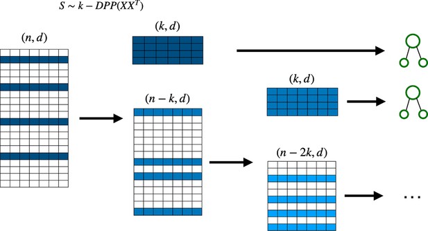
Deterministic determinantal point processes (DPP) sampling procedure for training decision trees.
At each step, a decision tree is trained usingthe sample that corresponds to the highest determinantal probability, and which is then removed from the original batch before continuing to the next decision tree.

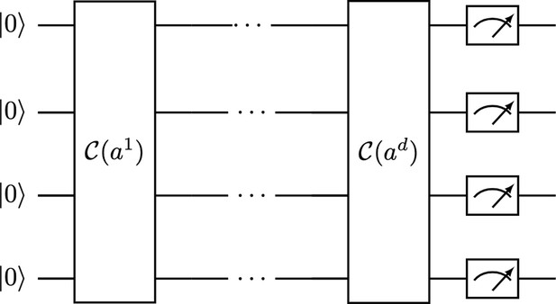
Types of data loaders.
Each line corresponds to a qubit. Each vertical line connecting two qubits corresponds to a reconfigurable beam splitter (RBS) gate. We also use gates. The depth of the first two loaders is linear, and the last one is logarithmic on the number of qubits.
Tables
AUC results for the SYNTH and MIMIC-III datasets, with MCAR and MNAR missingness, three holdout sets, and six different imputation methods.
Values are expressed as mean ± SD of 10 values for each experiment. DPP-MICE and detDPP-MICE are in bold when outperforming MICE and the underlined one is the best of the three. DPP-MissForest and detDPP-MissForest are in bold when outperforming MissForest and the underlined one is the best of the three.
| Dataset | Missingness | Set | MICE | DPP-MICE | detDPP-MICE | MissForest | DPP-MissForest | detDPP-MissForest |
|---|---|---|---|---|---|---|---|---|
| SYNTH | MCAR | H1 | 0.8318 ± 0.0113 | 0.835 ± 0.0083 | 0.8352 | 0.8525 ± 0.0044 | 0.8552 ± 0.0049 | 0.8582 |
| H2 | 0.8316 ± 0.008 | 0.8369 ± 0.0128 | 0.84 | 0.8465 ± 0.0057 | 0.849 ± 0.003 | 0.8491 | ||
| H3 | 0.8205 ± 0.0127 | 0.8266 ± 0.0096 | 0.8272 | 0.8436 ± 0.0031 | 0.8452 ± 0.0048 | 0.855 | ||
| MNAR | H1 | 0.8903 ± 0.0046 | 0.8915 ± 0.007 | 0.8934 | 0.7133 ± 0.0063 | 0.7171 ± 0.01 | 0.7185 | |
| H2 | 0.8755 ± 0.01 | 0.8745 ± 0.0072 | 0.8955 | 0.7052 ± 0.0036 | 0.7124 ± 0.0078 | 0.7167 | ||
| H3 | 0.9003 ± 0.0059 | 0.9005 ± 0.006 | 0.9041 | 0.769 ± 0.0103 | 0.7773 ± 0.0129 | 0.7905 | ||
| MIMIC | MCAR | H1 | 0.7621 ± 0.0046 | 0.7628 ± 0.0049 | 0.7641 | 0.7687 ± 0.0012 | 0.77 ± 0.0013 | 0.771 |
| H2 | 0.7541 ± 0.0037 | 0.7532 ± 0.0047 | 0.7619 | 0.7649 ± 0.0019 | 0.777 ± 0.0019 | 0.7707 | ||
| H3 | 0.7365 ± 0.0055 | 0.7394 ± 0.0052 | 0.7471 | 0.7485 ± 0.001 | 0.7507 ± 0.0017 | 0.7515 | ||
| MNAR | H1 | 0.77 ± 0.0026 | 0.7717 ± 0.0036 | 0.7722 | 0.6616 ± 0.0065 | 0.6715 ± 0.07 | 0.6760 | |
| H2 | 0.777 ± 0.0064 | 0.7818 ± 0.0029 | 0.7812 | 0.6748 ± 0.0045 | 0.6778 ± 0.0048 | 0.6798 | ||
| H3 | 0.7324 ± 0.0047 | 0.7363 ± 0.0031 | 0.7403 | 0.6368 ± 0.0034 | 0.64 ± 0.004 | 0.6419 |
-
AUC = area under the receiver operating curve; MCAR = missing completely at random; MNAR = missing not at random.
AUC results on the different holdout sets after imputation using MICE, DPP-MICE, and detDPP-MICE.
In the case of MICE and DPP-MICE, the boxplots correspond to 10 AUC values for 10 iterations of the same imputation and classification algorithms, depicting the lower and upper quartiles as well as the median of these 10 values. The AUC values are the same for every iteration of the detDPP-MICE algorithm.
| MCAR | MNAR | |
|---|---|---|
| SYNTH | 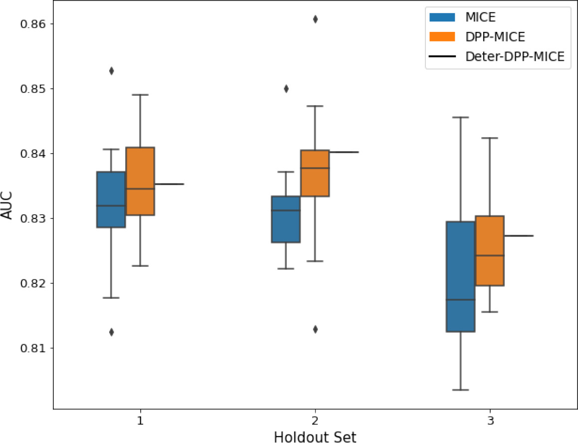 |  |
| MIMIC | 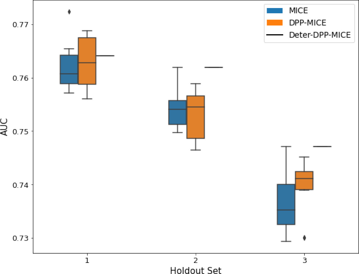 | 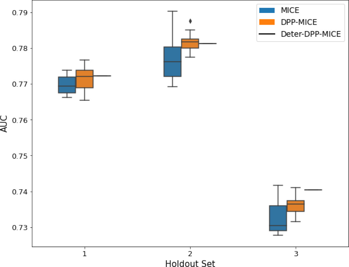 |
-
AUC = area under the receiver operating curve; MCAR = missing completely at random; MNAR = missing not at random.
AUC results on the different holdout sets after imputation using MissForest, DPP-MissForest, and detDPP-MissForest.
In the case of MissForest and DPP-MissForest, the boxplots correspond to 10 AUC values for 10 iterations of the same imputation and classification algorithm, depicting the lower and upper quartiles as well as the median of these 10 values. The AUC values are always the same for every iteration of the detDPP-MissForest algorithm.
| MCAR | MNAR | |
|---|---|---|
| SYNTH | 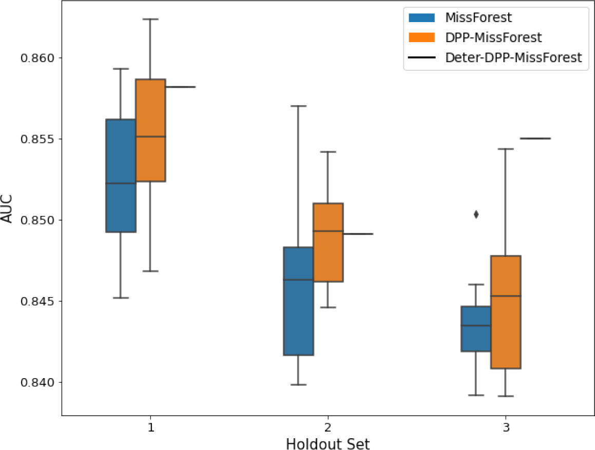 | 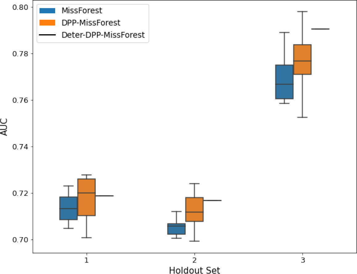 |
| MIMIC |  | 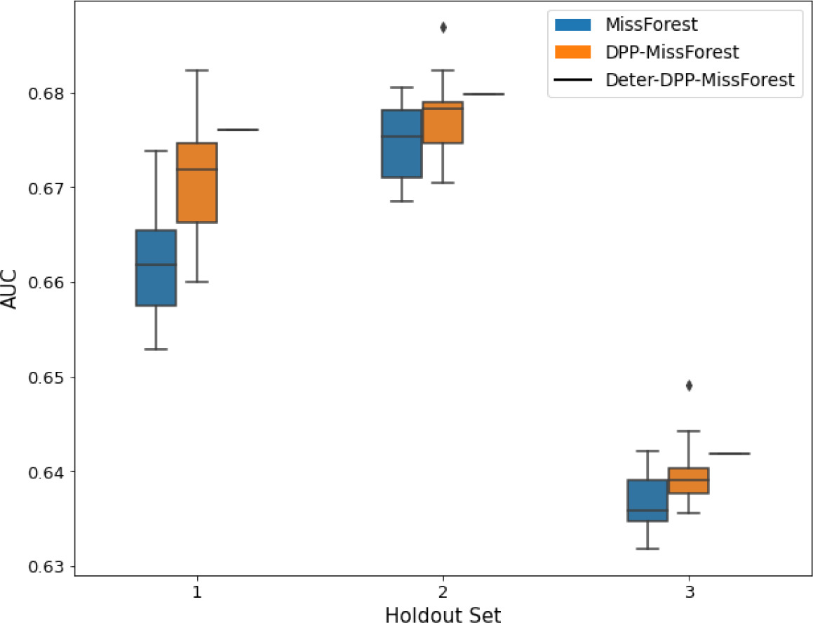 |
-
AUC = area under the receiver operating curve; MCAR = missing completely at random; MNAR = missing not at random.
Data matrix sizes used by the quantum determinantal point processes (DPP) circuits to train each tree.
The number of rows corresponds to the number of data points and is equal to the number of qubits of every circuit.
| Batch size | Tree 1 | Tree 2 | Tree 3 | Tree 4 |
|---|---|---|---|---|
| 7 | (7,2) | (5,2) | - | - |
| 8 | (8,2) | (6,2) | (4,2) | - |
| 10 | (10,2) | (8,2) | (6,2) | (4,2) |
Hardware results using the IBM quantum processor, depicting AUC results of the downstream classifier task after imputing missing values using DPP-MissForest.
In the case of MissForest and the quantum hardware DPP-MissForest implementations, the boxplots correspond to 10 AUC values for 10 iterations of the same imputation and classification algorithm, depicting the lower and upper quartiles as well as the median of these 10 values. The AUC values are the same for every iteration of the quantum DPP-MissForest algorithm using the simulator.
| Batch size: 7Number of trees: 2 | Batch size: 8Number of trees: 3 | Batch size: 10Number of trees: 4 | |
|---|---|---|---|
| MCAR SYNTH | 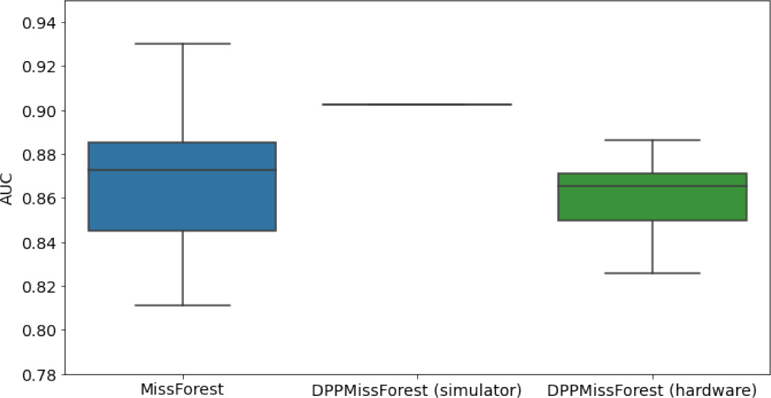 | 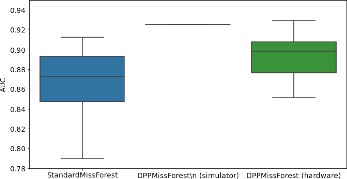 | 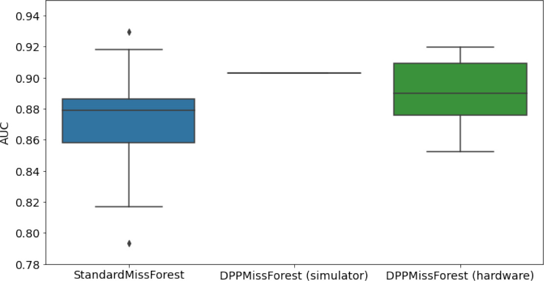 |
| MCAR MIMIC | 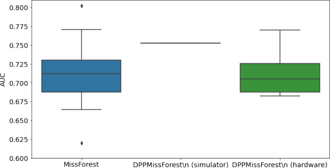 | 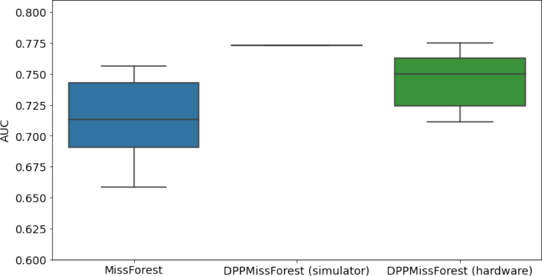 |  |
| MNAR SYNTH | 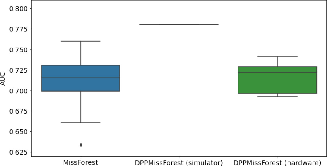 | 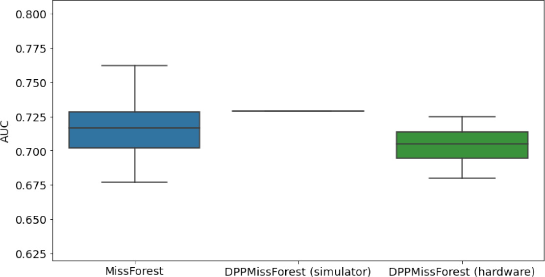 |  |
| MNAR MIMIC | 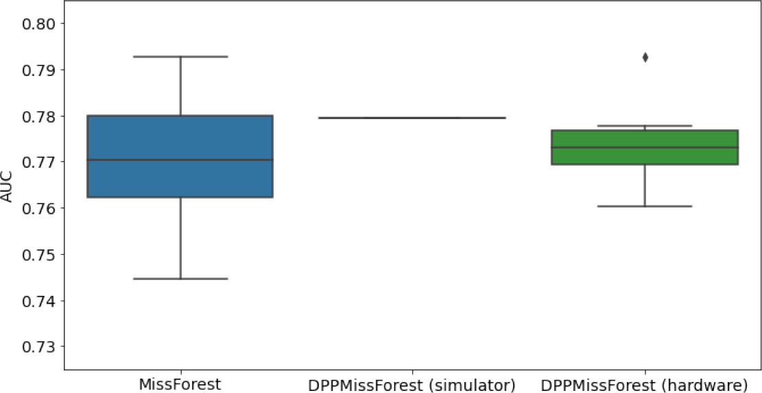 | 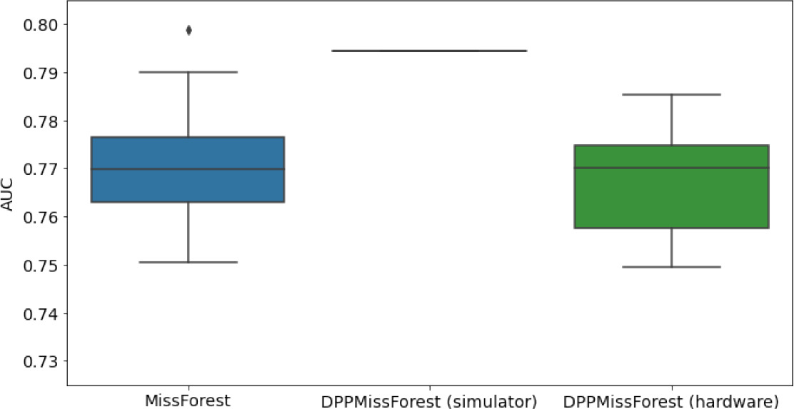 |  |
-
AUC = area under the receiver operating curve; MCAR = missing completely at random; MNAR = missing not at random.
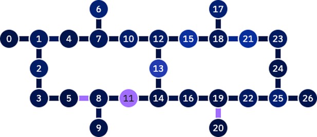
Numerical quantum hardware results showing the AUC results of the downstream classifier task on reduced datasets.
Values are represented according to mean ± SD format given 10 values for each experiment.
| Dataset | Missingness | Batch size | Trees | MissForest | detDPP-MissForest (simulator) | detDPP-MissForest (hardware) |
|---|---|---|---|---|---|---|
| SYNTH | MCAR | 7 | 2 | 0.868 ± 0.0302 | 0.9026 | 0.8598 ± 0.021 |
| 8 | 3 | 0.8667 ± 0.0342 | 0.9256 | 0.8923 ± 0.027 | ||
| 10 | 4 | 0.8725 ± 0.0275 | 0.9028 | 0.8902 ± 0.024 | ||
| MNAR | 7 | 2 | 0.7122 ± 0.0264 | 0.78 | 0.7149 ± 0.02 | |
| 8 | 3 | 0.7153 ± 0.022 | 0.729 | 0.7036 ± 0.0167 | ||
| 10 | 4 | 0.7258 ± 0.0157 | 0.7868 | 0.7082 ± 0.036 | ||
| MIMIC | MCAR | 7 | 2 | 0.7127 ± 0.038 | 0.7522 | 0.7117 ± 0.0315 |
| 8 | 3 | 0.7136 ± 0.03 | 0.7728 | 0.7448 ± 0.0258 | ||
| 10 | 4 | 0.6968 ± 0.03 | 0.7327 | 0.7262 ± 0.0299 | ||
| MNAR | 7 | 2 | 0.7697 ± 0.0133 | 0.7794 | 0.7742 ± 0.0108 | |
| 8 | 3 | 0.7713 ± 0.0112 | 0.7943 | 0.767 ± 0.0125 | ||
| 10 | 4 | 0.7712 ± 0.0116 | 0.7922 | 0.7675 ± .01545 |
-
AUC = area under the receiver operating curve; MCAR = missing completely at random; MNAR = missing not at random.
Summary of the characteristics of the different quantum determinantal point processes (DPP) circuits.
NN = nearest neighbor connectivity.
| Clifford loader | Hardware connectivity | Depth | # of RBS gates |
|---|---|---|---|
| Diagonal | NN | 2nd | 2nd |
| Semi-diagonal | NN | nd | 2nd |
| Parallel | All-to-all | 4d log(n) | 2nd |
Complexity comparison of d-DPP sampling algorithms, both classical (Mahoney et al., 2019) and quantum (Kerenidis and Prakash, 2022).
The problem considered is DPP sampling of rows from an matrix, where . For the quantum case, we provide both the depth and the size of the circuits.
| Classical | Quantum | |
|---|---|---|
| Preprocessing | ||
| Sampling |
-
DPP = determinantal point processes.


