Asymmetric distribution of color-opponent response types across mouse visual cortex supports superior color vision in the sky
- Department of Ophthalmology, Byers Eye Institute, Stanford University School of Medicine, United States
- Stanford Bio-X, Stanford University, United States
- Wu Tsai Neurosciences Institute, Stanford University, United States
- Department of Neuroscience & Center for Neuroscience and Artificial Intelligence, Baylor College of Medicine, United States
- Institute for Ophthalmic Research, University of Tübingen, Germany
- Graduate Training Center of Neuroscience, International Max Planck Research School, University of Tübingen, Germany
- Hertie Institute for AI in Brain Health, University of Tübingen, Germany
- Department of Electrical Engineering, Stanford University, United States
Figures
Figure 1 with 3 supplements
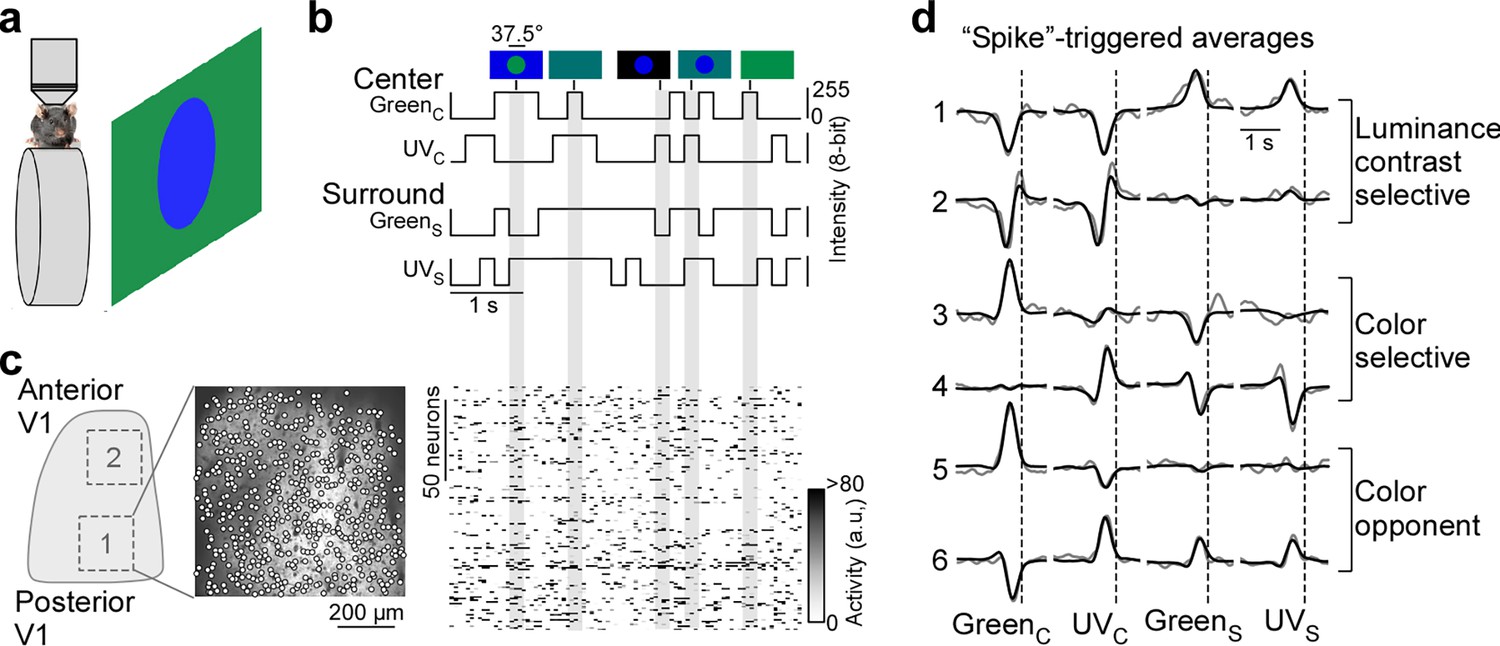
Color noise stimulus identifies center-surround receptive field properties of mouse primary visual cortex (V1) neurons.
(a) Schematic illustrating experimental setup: Awake, head-fixed mice on a treadmill were presented with a center-surround color noise stimulus while recording the population calcium activity in L2/3 neurons of V1 using two-photon imaging. Stimuli were back-projected on a Teflon screen by a DLP-based projector equipped with a ultraviolet (UV) (390 nm) and green (460 nm) LED, allowing to differentially activate mouse cone photoreceptors. (b) Schematic drawing illustrating stimulus paradigm: UV and green center spot (UVC /GreenC) and surround annulus (UVS /GreenS) flickered independently at 5 Hz according to binary random sequences. Top images depict example stimulus frames. See also Figure 1—figure supplement 1. (c) Left side shows a schematic of V1 with a posterior and anterior recording field, and the recorded neurons of the posterior field overlaid on top of the mean projection of the recording. Right side shows the activity of n=150 neurons of this recording in response to the stimulus sequence shown in (b). (d) Event-triggered averages (ETAs) of six example neurons, shown for the four stimulus conditions. Gray: Original ETA. Black: Reconstruction using principal component analysis (PCA). See also Figure 1—figure supplement 2. Cells are grouped based on their ETA properties and include luminance-sensitive, color selective, and color-opponent neurons. Black dotted lines indicate time of response.
Figure 1—figure supplement 1
Verification of stimulus paradigm.
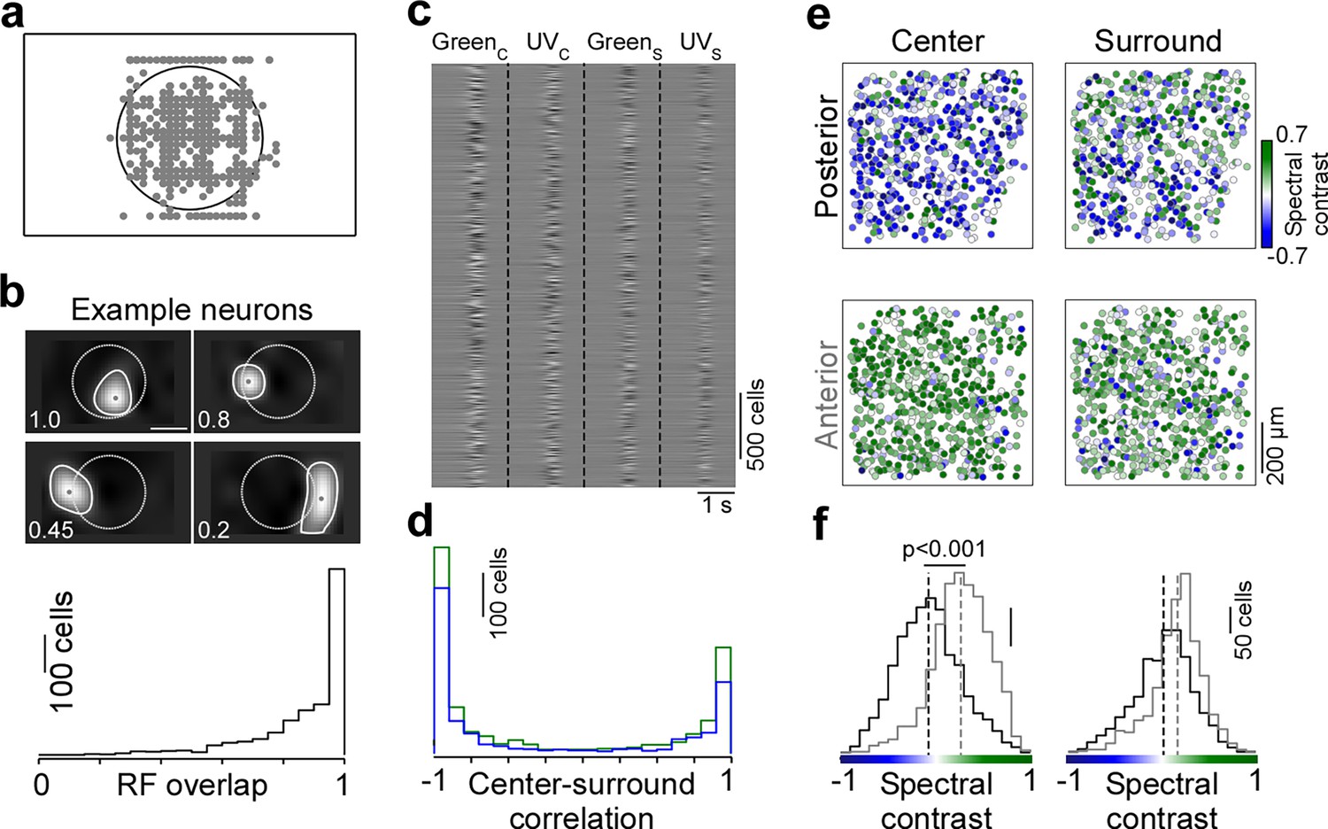
(a) Peak positions of spatial event-triggered averages (ETAs) estimated in response to a sparse noise stimulus (n=1434 cells, n=5 recording field, n=3 mice) relative to area of center spot of color noise stimulus (black). The peak position of the vast majority of cells lies within the center spot area. (b) Peak-normalized spatial ETA of four example neurons, capturing the center receptive field (RF) of the neurons. White solid line shows spatial ETA border (contour drawn at level = 0.25) and gray dot corresponds to peak of spatial ETA (see (a)). White dotted line indicates area of center spot of color noise stimulus shown in Figure 1. Overlap values depict the overlap of the spatial ETA with the center spot area, ranging from 1 (spatial ETA lies within the center spot area) to 0 (spatial ETA outside center spot area). Bottom shows distribution of spatial ETA overlap values (n=1434 cells, n=5 recording field, n=3 mice). For most cells (83%), the spatial ETA exhibited an overlap with the center spot area of the color noise stimulus of more than 0.65. (c) Principal component analysis (PCA)-reconstructed ETAs of all neurons above quality threshold (n=3331 cells, n=6 recording fields, n=3 mice). (d) Distribution of Pearson correlation coefficients of center and surround ETAs, estimated by correlating center and surround ETAs for the ultraviolet (UV) (blue) and green stimulus condition, respectively. (e) Neurons recorded in a posterior and anterior recording field of an example mouse, color-coded based on the cells’ color preference for center (left) and surround ETA (right), quantified as spectral contrast. (f) Distribution of center (left) and surround ETA (right) spectral contrast values for posterior (black; n=1616 cells) and anterior (gray; n=1695 cells) neurons from n=3 mice. Spectral contrast significantly differed between posterior and anterior neurons, for both center (p<0.001, two-sided two-sample t-test) and surround (p<0.001, two-sided two-sample t-test). Spectral contrast significantly differed between center and surround, for both posterior (p<0.001, two-sided two-sample t-test) and anterior neurons (p<0.001, two-sided two-sample t-test).
Figure 1—figure supplement 2
Event-triggered averages (ETAs) and quality control.
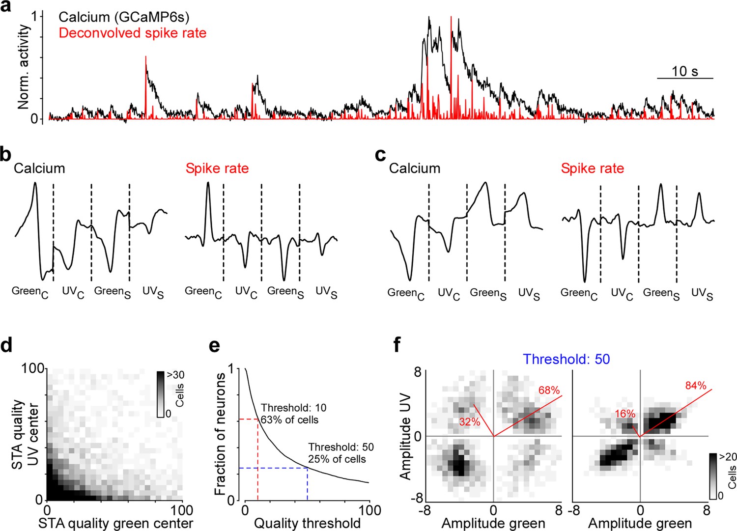
(a) Raw calcium trace (black) and trace deconvolved with the calcium sensor’s decay function (red) for one example neuron. (b) ETAs estimated based on raw (left) and deconvolved calcium traces (right), respectively, for one example neuron. (c) Same as (c) but for another example neuron. (d) Histogram of quality measure for green center ETA versus ultraviolet (UV) center ETA. The quality measure indicates the ratio of ETA to baseline variance (the higher the better quality). (e) Fraction of neurons above quality threshold, for varying quality thresholds. All analyses were performed for neurons with a UV or green center ETA quality >10 (red), corresponding to 63% of neurons. The blue indicates a more conservative threshold (>50), corresponding to only the the best 25% of neurons. (f) Density plot of peak amplitudes of center (left) and surround (right) ETAs across all neurons above conservative threshold (blue in (e)). Red lines correspond to axes of principal components (PCs) obtained from a principal component analysis (PCA) on the center or surround data, with percentage of variance explained along the polarity and color axis indicated.
Figure 1—figure supplement 3
Reconstruction of event-triggered averages (ETAs) using sparse principal component analysis (PCA).
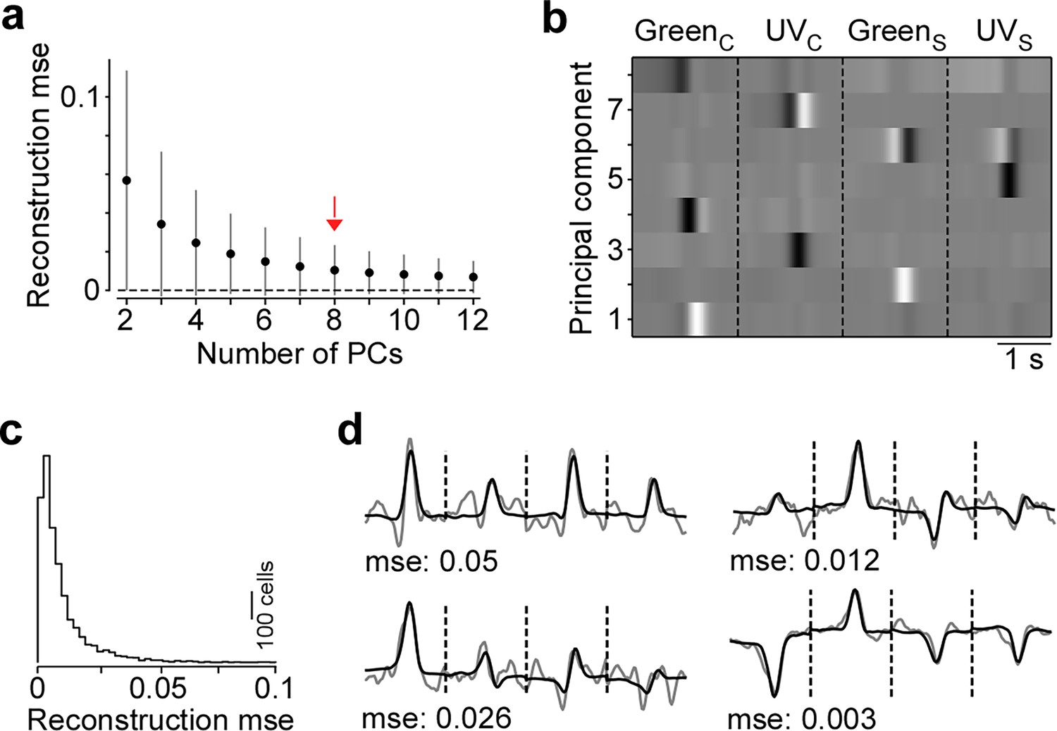
(a) Mean reconstruction error across neurons (s.d. in gray) quantified as mean squared error (mse) between the original ETA and the reconstruction using sparse PCA for varying numbers of principal components (PCs). For further analysis, we used sparse PCA with eight PCs, because (i) adding more PCs only slightly decreased reconstruction error and (ii) PCs ETArted to capture noise. (b) PCs obtained from sparse PCA on the ETAs (c) used for reconstructions. (c) Distribution of reconstruction mse values for sparse PCA with eight PCs. (d) Original ETA (gray) and PCA reconstruction (black) for four example neurons with varying mse.
Figure 2 with 2 supplements
Strong neuronal representation of color in mouse primary visual cortex.
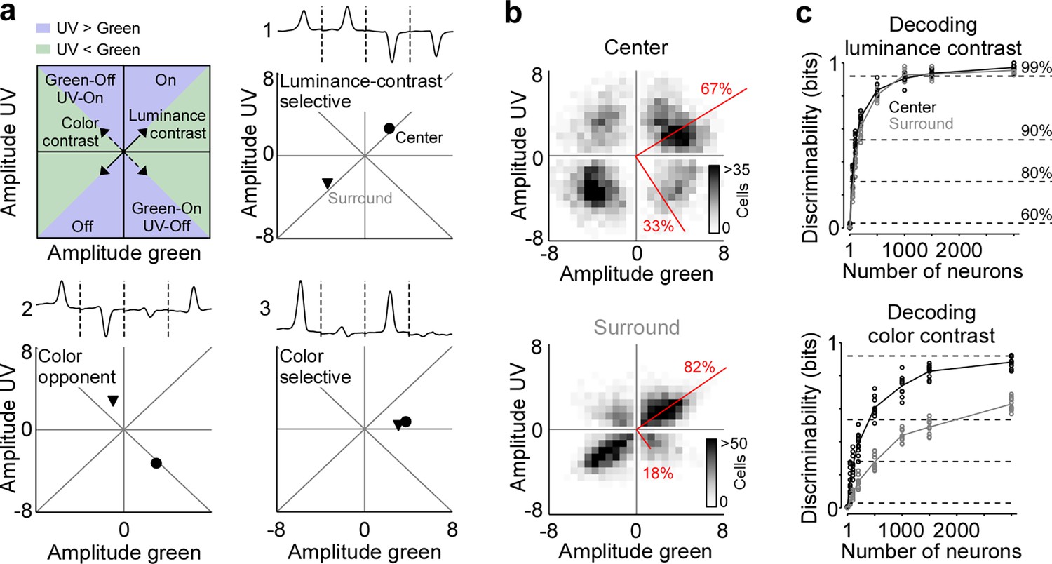
(a) Top left panel shows schematic drawing illustrating the green and ultraviolet (UV) contrast space used in the other panels and Figures 3—5. Amplitudes below and above zero indicates an Off and On cell, respectively. Achromatic On and Off cells will scatter in the lower left and upper right quadrants along the diagonal (‘luminance contrast‘), while color-opponent cells will fall within the upper left and lower right quadrants along the off-diagonal (‘color contrast‘). Blue and green shading indicates stronger responses to UV and green stimuli, respectively. The three other panels show event-triggered averages (ETAs) of three example neurons (top) with the peak amplitudes (‘contrast‘) of their center (dot) and surround responses (triangle) indicated in the bottom. (b) Density plot of peak amplitudes of center (top) and surround (bottom) ETAs across all neurons (n=3331 cells, n=6 recording fields, n=3 mice). Red lines correspond to axes of principal components (PCs) obtained from a principal component analysis (PCA) on the center or surround data, with percentage of variance explained along the polarity and color axis indicated. For reproducibility across animals, see Figure 2—figure supplement 1. The percentages of variance explained by color (off-diagonal) and luminance axis (diagonal) correlate with the number of neurons located in the color (top left and bottom right) and luminance contrast quadrants (top right and bottom left), respectively. Scale bars indicate the number of neurons in the 2D histogram. (c) Decoding discriminability of stimulus luminance (top) and stimulus color (bottom) based on center (black) and surround (gray) responses of different numbers of neurons. Decoding was performed using a support vector machine (SVM). Lines indicate the mean of 10-fold cross-validation (shown as dots). For luminance contrast, decoding discriminability was significantly different between center and surround for n=50 and n=100 neurons (t-test for unpaired data, p-value was adjusted for multiple comparisons using Bonferroni correction). For color contrast, decoding discriminability was significantly different between center and surround for all numbers of neurons tested, except n=1 neuron. Dotted horizontal lines indicate decoding accuracy in % for 60%, 80%, 90%, and 99%, with a change level of 50% corresponding to 0 bits.
Figure 2—figure supplement 1
Consistency across mice.
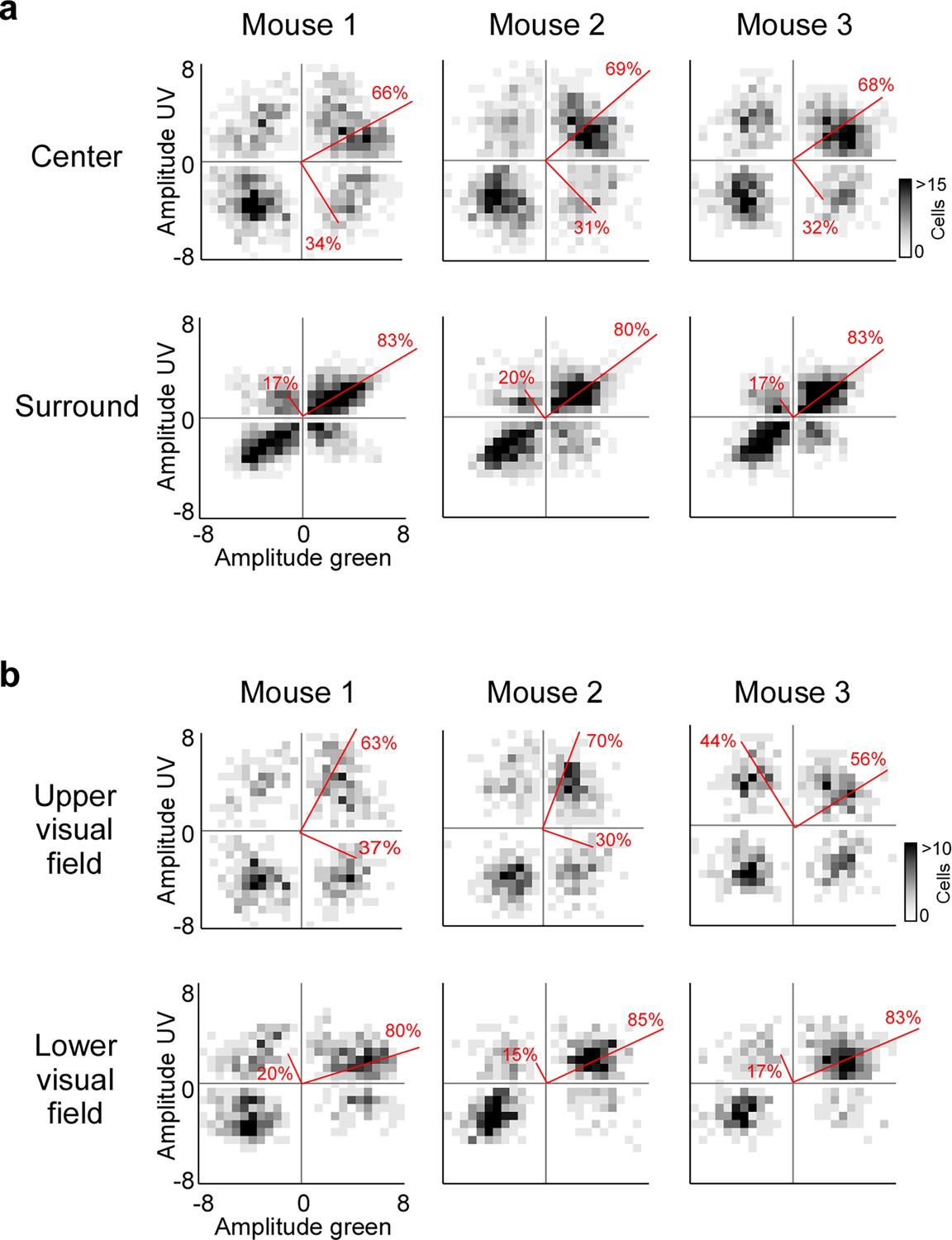
(a) Density plots of peak amplitudes of center (top) and surround (bottom) event-triggered averages (ETAs), separately for mouse 1 (n=2 recording fields, n=1170 cells), mouse 2 (n=2 recording fields, n=1102 cells), and mouse 3 (n=2 recording fields, n=1039 cells). Red lines correspond to axes of principal components (PCs) obtained from a principal component analysis (PCA) on the center or surround data, with percentage of variance explained along the polarity and color axis indicated. (b) Density plots of peak amplitudes of center ETAs for neurons encoding the upper visual field (posterior primary visual cortex [V1]; top) and lower visual field (anterior V1; bottom), respectively, separately for mouse 1 (n=2 recording fields, n=1170 cells), mouse 2 (n=2 recording fields, n=1102 cells), and mouse 3 (n=2 recording fields, n=1039 cells). Red lines correspond to axes of PCs obtained from a PCA on the center or surround data, with percentage of variance explained along the polarity and color axis indicated.
Figure 2—figure supplement 2
Neuronal representation of color in the mouse retina.
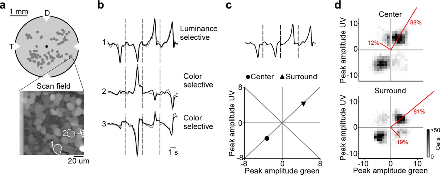
(a) Top panel shows schematic of a flat-mounted ex vivo retina, with distribution of all recording fields (n=88 fields) from an available dataset (Szatko et al., 2020) that has recorded the responses of ganglion cell layer (GCL) cells in response to center and surround flicker of ultraviolet (UV) and green LED. The bottom panel shows one example scan field of the GCL with 64×64 pixels, recorded at 7.8 Hz. The cells indicated with numbers are shown in panel (b). D: dorsal, T: temporal. (b) Event-triggered averages (ETAs) of three example neurons, concatenated across the four stimulus conditions (center and surround for UV and green flicker). Gray: Original ETA. Black: Reconstruction using principal component analysis (PCA). Similar to primary visual cortex (V1), there are luminance-sensitive neurons (cell 1) and color selective neurons (cells 2 and 3). In contrast to V1, color-opponent neurons were rare. (c) This panel shows the ETA of neuron 1 in (b), with its peak amplitudes of center and surround indicated in the luminance and contrast sensitivity space. (d) Density plot of peak amplitudes of center (top) and surround (bottom) ETAs across all retinal ganglion cell (RGC) (n=3215 cells, n=88 recording fields, n=18 mice). Red lines correspond to axes of principal components (PCs) obtained from a PCA on the center or surround data, with percentage of variance explained along the polarity and color axis indicated.
Figure 3
Reduced representation of color contrast in mouse primary visual cortex (V1) for lower ambient light levels.
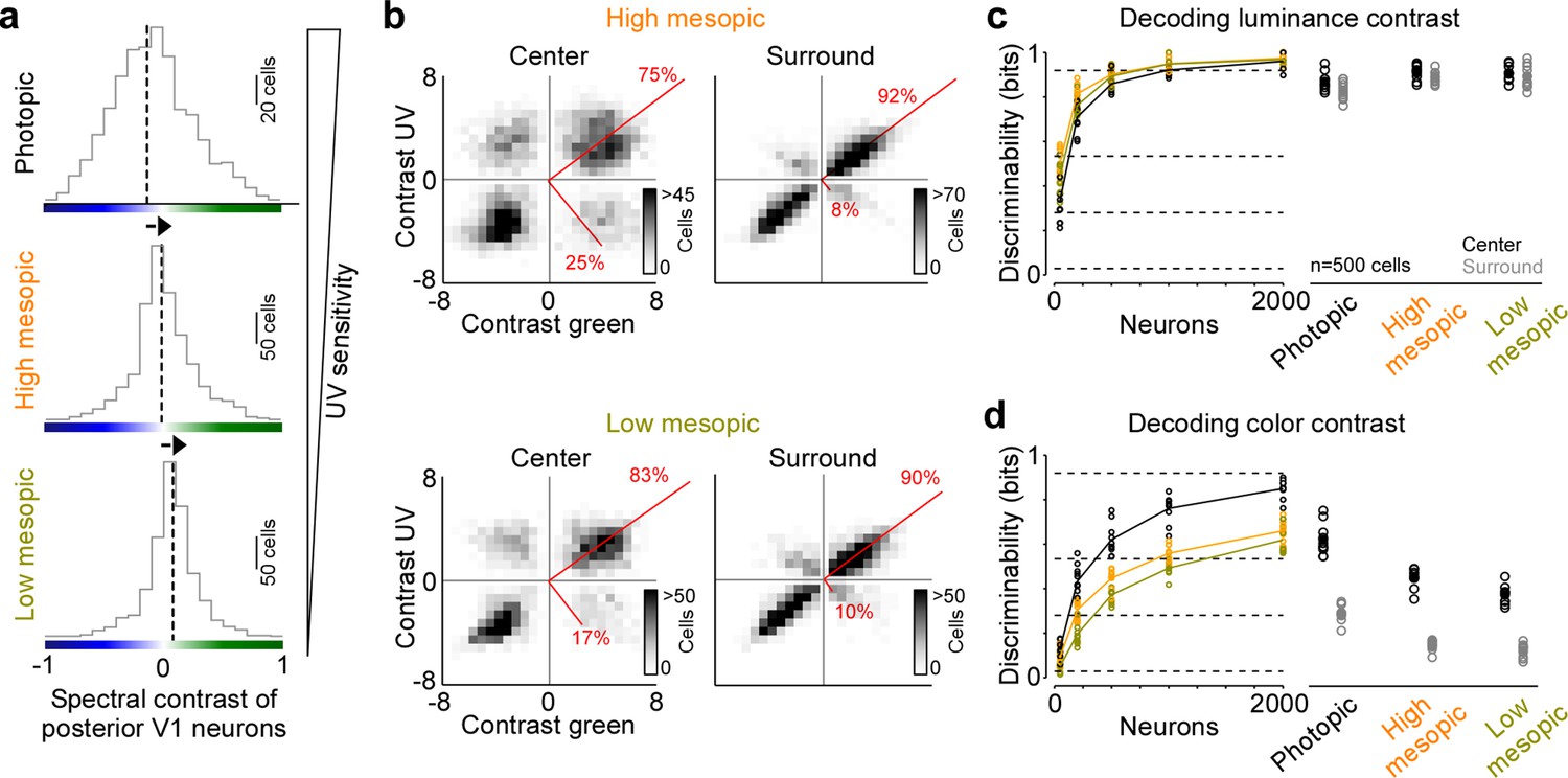
(a) Distribution of spectral contrast of center event-triggered averages (ETAs) of all neurons recorded in posterior V1, for photopic (top, n=1616 cells, n=3 recording fields, n=3 mice), high mesopic (middle, n=1485 cells, n=3 recording fields, n=3 mice), and low mesopic (bottom, n=1295 cells, n=3 recording fields, n=3 mice) ambient light levels. Black dotted lines indicate mean of distribution. Spectral contrast significantly differed across all combinations of light levels (t-test for unpaired data, p-value was adjusted for multiple comparisons using Bonferroni correction). The triangle on the right indicates ultraviolet (UV) sensitivity of the neurons, which is decreasing with lower ambient light levels. (b) Density plot of peak amplitudes of center (left) and surround (right) ETAs. Red lines correspond to axes of principal components (PCs) obtained from a principal component analysis (PCA) on the center or surround data, with percentage of variance explained along the polarity and color axis indicated. Top row shows high mesopic (n=3522 cells, n=6 recording fields, n=3 mice) and bottom row low mesopic (n=2705 cells, n=6 recording fields, n=3 mice) light levels. The percentages of variance explained by color (off-diagonal) and luminance axis (diagonal) correlate with the number of neurons located in the color (top left and bottom right) and luminance contrast quadrants (top right and bottom left), respectively. Scale bars indicate the number of neurons in the 2D histogram. (c) Discriminability (in bits) of luminance contrast (On versus Off) for the center across the three light levels tested, obtained from training support vector machine (SVM) decoders based on recorded noise responses of V1 neurons. Right plot shows the discriminability of luminance contrast for n=500 neurons for center and surround. Dots show decoding performance of 10 train/test trial splits. For n=500 neurons, decoding discriminability of the center was not significantly different across light levels (t-test for unpaired data, p-value was adjusted for multiple comparisons using Bonferroni correction). The surround discriminability was significantly lower than the center for the photopic condition. Dotted horizontal lines indicate decoding accuracy in % for 60%, 80%, 90%, and 99%, with a change level of 50% corresponding to 0 bits. (d) Like (c), but showing discriminability of color contrast (green versus UV). Decoding discriminability was significantly different between center and surround for all three light levels. In addition, discriminability for the center was significantly different between photopic and mesopic conditions, but not between the two mesopic conditions (t-test for unpaired data, p-value was adjusted for multiple comparisons using Bonferroni correction). Dotted horizontal lines indicate decoding accuracy in % for 60%, 80%, 90%, and 99%, with a change level of 50% corresponding to 0 bits.
Figure 4
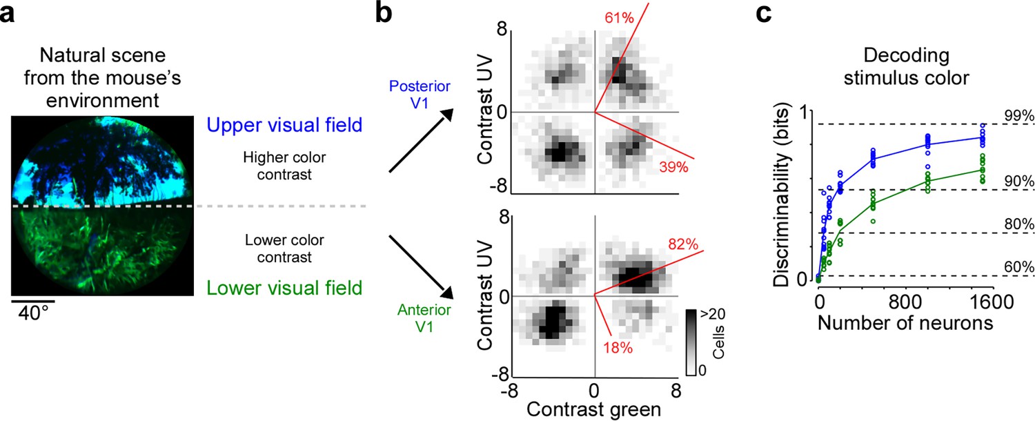
Cortical representation of color changes across visual space.
(a) Natural scene captured in the natural environment of mice using a custom-built camera adjusted to the mouse’s spectral sensitivity (Qiu et al., 2021). Dashed line indicates the horizon and separates the scene into lower and upper visual field. Previous studies Qiu et al., 2021; Abballe and Asari, 2022 have reported higher color contrast in the upper compared to the lower visual field. (b) Density plot of peak amplitudes of center event-triggered averages (ETAs) across neurons recorded in posterior (top) and anterior primary visual cortex (V1) (bottom). Red lines correspond to axes of principal components (PCs) obtained from a principal component analysis (PCA), with percentage of variance explained along the polarity and color axis indicated. For reproducibility across animals, see Figure 2—figure supplement 1. The percentages of variance explained by color (off-diagonal) and luminance axis (diagonal) correlate with the number of neurons located in the color (top left and bottom right) and luminance contrast quadrants (top right and bottom left), respectively. Scale bars indicate the number of neurons in the 2D histogram. (c) Discriminability (in bits) of color contrast (ultraviolet [UV] or green) for neurons recorded in posterior (blue) and anterior V1 (green), obtained from training support vector machine (SVM) decoders based on recorded noise responses of V1 neurons. The decoding discriminability was significantly different between anterior and posterior neurons (t-test for unpaired data, p-value was adjusted for multiple comparisons using Bonferroni correction). Dotted horizontal lines indicate decoding accuracy in % for 60%, 80%, 90%, and 99%, with a change level of 50% corresponding to 0 bits.
Figure 5 with 1 supplement
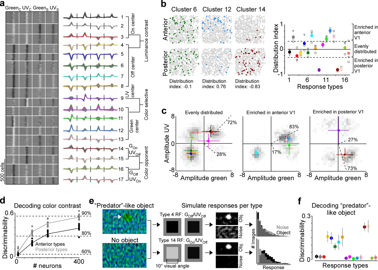
Asymmetric distribution of color response types explains higher color sensitivity in posterior primary visual cortex (V1).
(a) Clustering result of the Gaussian mixture model with n=17 clusters (see Figure 5—figure supplement 1 for details). Model input corresponded to the weights of the principal components used for reconstructing event-triggered averages (ETAs). Left panel shows ETAs of all cells, respectively, sorted by cluster assignment. Right panel shows mean ETA of each cluster (s.d. shading in gray). Clusters are sorted based on broad response categories, which are indicated on the right. (b) Left shows distribution of cells assigned to three different clusters (color) in a posterior and anterior recording field of one example animal. Gray dots show cells assigned to other clusters. Distribution index for each cluster is indicated below. Right shows the mean distribution index per cluster, with different marker shapes indicating the indices for individual animals. Zero indicates an even distribution across anterior and posterior V1 and values above and below zero indicate that cells are enriched in anterior and posterior V1, respectively. Dotted horizontal lines at –0.33/0.33 indicate twice as many cells in posterior than anterior cortex and vice versa. (c) Histograms of peak amplitudes of center ETAs for clusters that are evenly distributed across V1 (left, distribution index >–0.33 and <0.33), enriched in anterior V1 (middle, distribution index) and enriched in posterior V1 (right). Cluster means and s.d. are indicated in color. Dotted lines correspond to axes of PCs obtained from a principal component analysis (PCA), with percentage of variance explained along the luminance and color axis indicated. The percentages of variance explained by color (off-diagonal) and luminance axis (diagonal) correlate with the number of neurons located in the color (top left and bottom right) and luminance contrast quadrants (top right and bottom left), respectively. Scale bars indicate the number of neurons in the 2D histogram. (d) Discriminability (in bits) of stimulus color contrast based on response types enriched in anterior (black) and posterior (gray) V1. Dots show decoding performance across 10 train/test trial splits. Decoding discriminability was significantly different between anterior- and posterior-enriched types for all numbers of neurons tested (t-test for unpaired data, p-value was adjusted for multiple comparisons using Bonferroni correction). Dotted horizontal lines indicate decoding accuracy in % for 60%, 80%, and 90%, with a change level of 50% corresponding to 0 bits. (e) Noise images with or without a ‘predator‘-like dark object in the UV channel were convolved with simulated center receptive fields (RFs), depicting the mean amplitudes of the green and UV center ETA per response type (shown for types 4 and 14). The resulting activity maps were summed and thresholded to simulate responses to n=1000 noise and object scenes. (f) Discriminability (in bits) of the presence of a ‘predator’-like dark object in the UV channel per response type. Error bars show s.d. across 10 train/test trial splits.
Figure 5—figure supplement 1
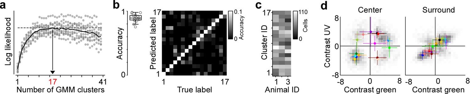
Unsupervised clustering of spike-triggered averages.
(a) Log likelihood of Gaussian mixture models (GMMs) with varying numbers of clusters. Model input corresponded to the weights of the principal components used for reconstructing event-triggered averages (ETAs) (Figure 1—figure supplement 3). Black solid trace corresponds to the mean across 10 train/test data splits (gray dots). Black dotted trace indicates maximum log likelihood for n=17 clusters. (b) Box plot shows distribution of assignment accuracy across clusters, obtained from comparing ground-truth labels generated using mean and covariance matrix of each Gaussian (i.e. cluster) with labels predicted by the pre-trained GMM (see also Tolias et al., 2007). Right panel shows confusion matrix of true versus predicted labels. Please note that false positives are usually across clusters with similar response properties. (c) Number of cells assigned to the different clusters, sorted by animal. d, scatter plot of peak amplitudes of center (top) and surround (bottom) ETAs across all neurons, with mean and s.d. of each cluster from Figure 5a indicated in color.
Additional files
Download links
A two-part list of links to download the article, or parts of the article, in various formats.
Downloads (link to download the article as PDF)
Open citations (links to open the citations from this article in various online reference manager services)
Cite this article (links to download the citations from this article in formats compatible with various reference manager tools)
Asymmetric distribution of color-opponent response types across mouse visual cortex supports superior color vision in the sky
eLife 12:RP89996.
https://doi.org/10.7554/eLife.89996.4


