Representational drift as a result of implicit regularization
Figures
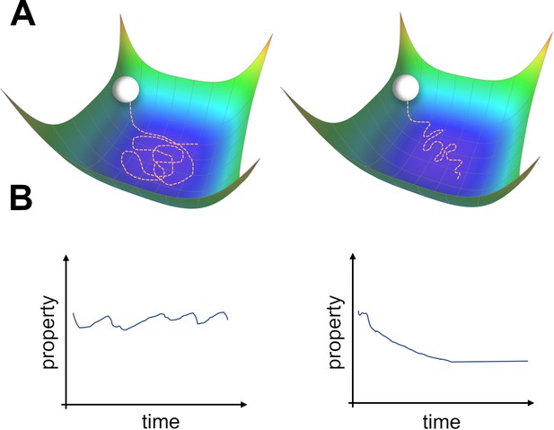
Two types of possible movements within the solution space.
(A) Two options of how drift may look in the solution space. Random walk within the space of equally good solutions that is either undirected (left) or directed (right). (B) The qualitative consequence of the two movement types. For an undirected random walk, all properties of the solution will remain roughly constant (left). For the directed movement there should be a given property that is gradually increasing or decreasing (right).
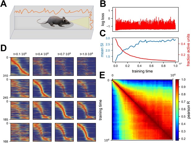
Continuous noisy learning leads to drift and spontaneous sparsification.
(A) Illustration of an agent in a corridor receiving high-dimensional visual input from the walls. (B) Loss as a function of training steps (log scale). Zero loss corresponds to a mean estimator. Note the rapid drop in loss at the beginning, after which it remains roughly constant. (C) Mean spatial information (SI, blue) and fraction of units with non-zero activation for at least one input (red) as a function of training steps. (D) Rate maps sampled at four different time points (columns). Maps in each row are sorted according to a different time point. Sorting is done based on the peak tuning value to the latent variable. (E) Correlation of rate maps between different time points along training. Only active units are used.

Experimental data consistent with simulations.
Data from four different labs show sparsification of CA1 spatial code, along with an increase in the information of active cells. Values are normalized to the first recording session in each experiment. Error bars show standard error of the mean. (A) Fraction of place cells (slope=-0.0003 p < .001) and mean spatial information (SI) (slope=0.002, p < .001) per animal over 200 min (Khatib et al., 2023). (B) Number of cells per animal (slope=-0.052, p = .004) and mean SI (slope=0.094, p < .001) over all cells pooled together over 10 days. Note that we calculated the number of active cells rather than fraction of place cells because of the nature of the available data (Jercog et al., 2019b). (C) Fraction of place cells (slope=-0.048, p = .011) and mean SI per animal (slope=0.054, p < .001) over 11 days (Karlsson and Frank, 2008). (D) Fraction of place cells (slope=-0.026, p < .001) and mean SI (slope=0.068, p < .001) per animal over 8 days (Sheintuch et al., 2023).
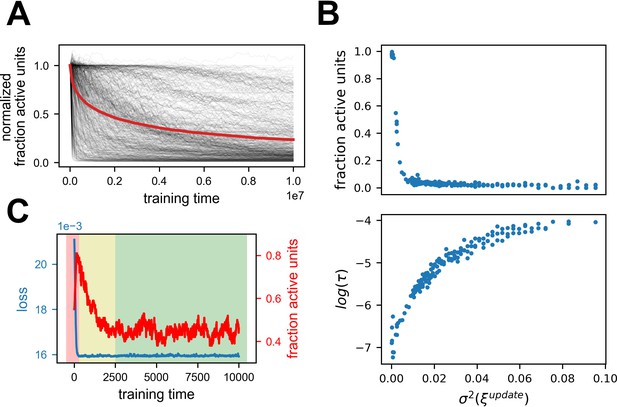
Generality of the results.
Summary of 616 simulations with various parameters, excluding stochastic gradient descent (SGD) with label noise (see Table 2). (A) Fraction of active units normalized by the first timestep for all simulations. Red line is the mean. Note that all simulations exhibit a stochastic decrease in the fraction of active units. See Figure 4—figure supplement 1 for further breakdown. (B) Dependence of sparseness (top) and sparsification time scale (bottom) on noise amplitude. Each point is one of 178 simulations with the same parameters except noise variance. (C) Learning a similarity matching task with Hebbian and anti-Hebbian learning using published code from Qin et al., 2023. Performance of the network (blue) and fraction of active units (red) as a function of training steps. Note that the loss axis does not start at zero, and the dynamic range is small. The background colors indicate which phase is dominant throughout learning (1 - red, 2 - yellow, 3 - green).

Noisy learning leads to spontaneous sparsification.
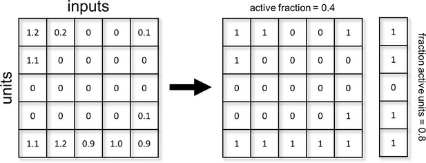
Summary of 516 simulations with three different learning algorithms: Stochastic error descent (SED, Cauwenberghs, 1992), SGD, Adam. All values are normalized to the first time step of each simulation. The red lines indicate mean over all simulations. (A) Fraction active units – number of units with any response. (B) Active fraction – overall activity across all units (see methods).

Noisy learning leads to a flat landscape.
(A) Gradient Descent dynamics over a two-dimensional loss function with a one-dimensional zero-loss manifold (colors from blue to yellow denote loss). Note that the loss is identically zero along the horizontal axis, but the left area is flatter. The orange trajectory begins at the red dot. Note the asymmetric extension into the left area. (B) Fraction of active units is highly correlated with the number of non-zero eigenvalues of the Hessian. (C) Update noise reduces small eigenvalues. Log of non-zero eigenvalues at two consecutive time points for learning with update noise. Note that eigenvalues do not correspond to one another when calculated at two different time points, and this plot demonstrates the change in their distribution rather than changes in eigenvalues corresponding to specific directions. The distribution of larger eigenvalues hardly changes, while the distribution of smaller eigenvalues is pushed to smaller values. (D) Label noise reduces the sum over eigenvalues. Same as (C), but for actual values instead of log.
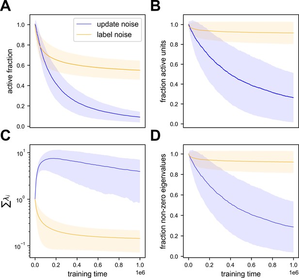
Label and update noise impose different regularization over the Hessian with distinct signatures in activity statistics.
Summary of 362 simulations with either label or update noise added to stochastic gradient descent (SGD) learning algorithm. All values are normalized to the first time step of each simulation. Lines indicate the mean of simulations and shaded regions indicate one standard deviation. Loss convergence varies between simulations, and is achieved on a scale of no more than 105 time steps. (A) Active fraction as a function of training time. Note this metric decreases significantly for both types of noise. (B) Fraction of active units as a function of training time. For label noise, the change is much smaller. (C) Sum of the loss Hessian’s eigenvalues as a function of training time. Here the difference is apparent - label noise imposes slow implicit regularization over this metric while update noise does not. (D) Fraction of non-zero eigenvalues in the loss Hessian as a function of training time. As explained in the main text, update noise imposes implicit regularization over the sum of log-eigenvalues, which manifests as a zeroing of eigenvalues over time and thus a reduction in the fraction of active units.
Tables
The three phases of noisy learning.
| Phase | Duration | Performance | Activity statistics | Representations |
|---|---|---|---|---|
| learning of task | short | changing | changing | changing |
| directed drift | long | stationary | changing | changing |
| null drift | endless | stationary | stationary | changing |
Parameter ranges for random simulations.
| Parameter | Possible values |
|---|---|
| learning algorithm | {SGD, Adam, SED} |
| noise type | {update, label} |
| number of samples | O’keefe and Nadel, 1979; Susman et al., 2019 |
| initialization regime | {lazy, rich} |
| task | {abstract predictive, random, random smoothed} |
| input dimension | O’keefe and Nadel, 1979; Susman et al., 2019 |
| output dimension | O’keefe and Nadel, 1979; Susman et al., 2019 |
| noise variance (label/update) | [0.1,1]/[0.01,0.1] |
| hidden layer size | 100 |
Description of experimental datasets.
| Khatib et al., 2023 | Jercog et al., 2019b | Karlsson et al., 2015 | Sheintuch et al., 2023 | Geva et al., 2023 | |
|---|---|---|---|---|---|
| Familiarity | 3–5 days | novel | novel | novel | 6–9 days |
| Species | mice | mice | rats | mice | mice |
| # Animals | 8 | 12 | 9 | 8 | 8 |
| Recordings days | 1 day | 10 days | max. 11 days | 10 days | 10 days |
| Session length | 200 min | 40 min | 15–30 min | 20 min | 20 min |
| Recording type | calcium imaging | electrophysiology | electrophysiology | calcium imaging | calcium imaging |
| Arena | linear track | square or circle | W-shaped | linear or L-shaped track | linear track |
| Activity metric | fraction of place cells decrease | number of active cells decrease | fraction of place cells decrease | fraction of place cells decrease | fraction of place cell stationary |
| Mean SI change | increase | increase | increase | increase | stationary |


