EEG-fMRI in awake rat and whole-brain simulations show decreased brain responsiveness to sensory stimulations during absence seizures
- University Grenoble Alpes, Inserm, U1216, Grenoble Institut Neurosciences, France
- A.I. Virtanen Institute for Molecular Sciences, University of Eastern Finland, Finland
- Paris-Saclay University, CNRS, Institut des Neurosciences (NeuroPSI), France, France
- University Grenoble Alpes, Inserm, US17, CNRS, UAR 3552, CHU Grenoble Alpes, IRMaGe, France
- Aix Marseille University, INSERM, INS, Inst Neurosci Syst, France
Figures
Figure 1 with 2 supplements
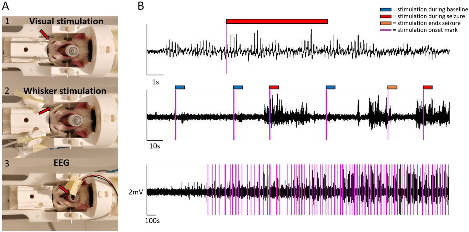
Sensory stimulation, EEG setup, and example EEG traces.
For visual stimulation, optical fiber cables were positioned bilaterally close to the eyes (A1) .For whisker stimulation, plastic tips guided air flow bilaterally to whiskers (A2). For EEG, carbon fiber leads were connected to electrodes coming from a plastic tube (A3). EEG traces are illustrated at three different temporal scale, during ictal and interictal states and with stimulation onset marks (B). Color tags mark stimulation onsets (purple) and the 6 s stimulation blocks during baseline (blue), seizure (red), and when stimulation ended a seizure (orange). The onset marks were added post hoc, based on recorded TTL events.
Figure 1—figure supplement 1

Example of EEG trace and illustration of stimulation and seizure block paradigms used as statistical parametric mapping (SPM) inputs.
Inputs (A) were convolved with third-order gamma functions (B), which was selected as basis functions, accounting for temporal and dispersion differences in hemodynamic responses. Example of translational and rotational motion parameters from one animal (C). Motion parameters were used as nuisance regressors and not convolved with a basis function.
Figure 1—figure supplement 2

Habituation and imaging schedules for three illustrative rats.
After 8 days of habituation, three to five functional magnetic resonance imaging (fMRI) experiment were conducted within a 1–3 week period for each rat. In case rats were re-imaged more than 1 week after the preceding experiment, an additional 2-day habituation period was conducted.
Figure 2 with 1 supplement
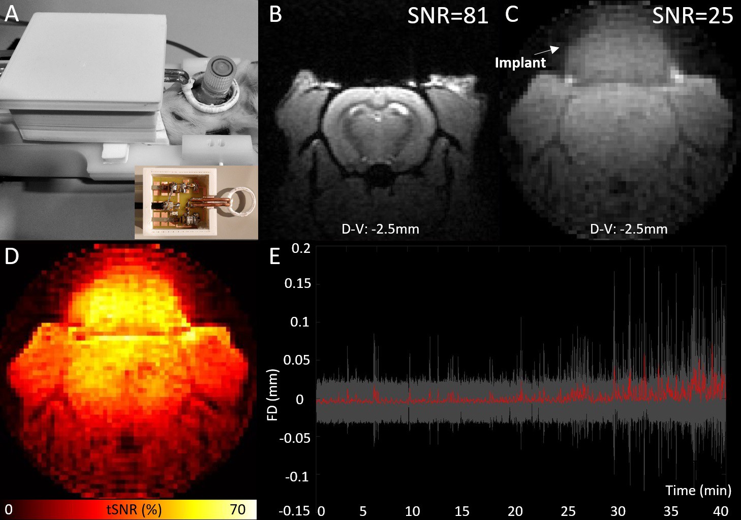
EEG-functional magnetic resonance imaging (fMRI) setup and illustration of MRI data quality.
MRI transmit-receive loop coil placed around the implant (A), spatial signal-to-noise ratios of an illustrative high-resolution T1-FLASH (B), and low-resolution zero echo time (ZTE) image (C), temporal signal-to-noise ratios (tSNRs) of ZTE data (D) from a one example animal and average framewise displacement (red) with the standard deviation (gray area) across all sessions included to analyses (E).
Figure 2—figure supplement 1
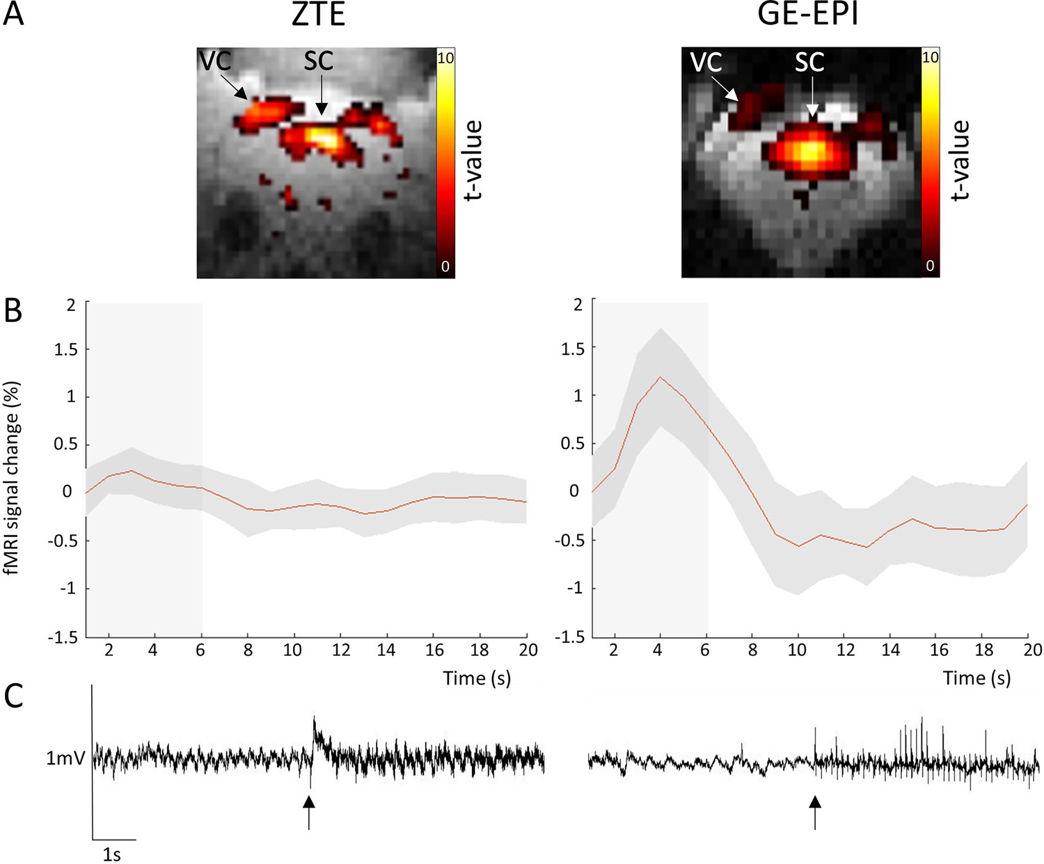
Zero echo time (ZTE) and gradient-echo-echo-planar imaging (GE-EPI) data collected during visual stimulus experiment (15s ON, 30s OFF paradigm), and EEG trace illustrating MRI gradient artifacts, from an example rat in preliminary study.
Illustration of image quality, and statistical t-contrast maps to visual stimulation (A), functional contrast (B), and effect of EEG artifact (C) for both imaging sequences. Although ZTE exhibits lower functional contrast compared to EPI sequence, it offered a better spatial brain coverage with less image distortions, thus yielding far better stimulation-induced maps. ZTE also caused relatively less artificial noise on EEG signal, keeping both amplitude of the signal and frequencies relatively more intact, which improved live detection of absence seizures. Gray box illustrates stimulation period. Arrows on EEG signal mark the beginning of each functional magnetic resonance imaging (fMRI) sequence.
Figure 3
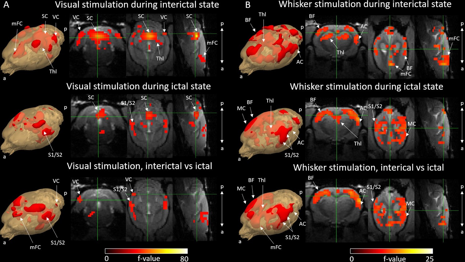
Activation F-contrast maps of stimulation responses during interictal and ictal states and difference maps between these two states for the visual (A) and the whisker (B) stimulation experiments.
Parameter estimates of regressors were calculated for every voxel, and contrasts were added to parameter estimates of interictal stimulation, ictal stimulation, and to compare interictal versus ictal stimulation in visual (A) and whisker (B) stimulation groups. For statistical significance, F-contrast (p<0.05) maps were created and corrected for multiple comparisons by cluster-level correction. AC = auditory cortex, BF = barrel field, mFC = medial frontal cortex, SC = superior colliculus, S1/S2 = primary and secondary somatosensory cortex, Thl = thalamus, VC = visual cortex. a = anterior, p = posterior.
Figure 4 with 1 supplement

Hemodynamic response functions (HRFs) to stimulations performed during an interictal and ictal period: visual stimulation (A) and whisker stimulation (B) groups.
HRFs were calculated in selected ROI, belonging to visual or somatosensory area, by multiplying gamma basis functions (Figure 1—figure supplement 1B) with its corresponding average beta-value over a ROI and taking a sum of these values. For statistical comparison, extreme beta-values over a ROI were calculated and values between two states were compared with a two-sample t-test (n=9 sesions in visual stimulation group, n=8 in whisker stimulation group). Scatter plot represents mean ± SD and each blue dot corresponds to extreme beta-values observed from individual functional magnetic resonance imaging (fMRI) sessions. ***=p<0.001. Gray box illustrates stimulation period.
Figure 4—figure supplement 1
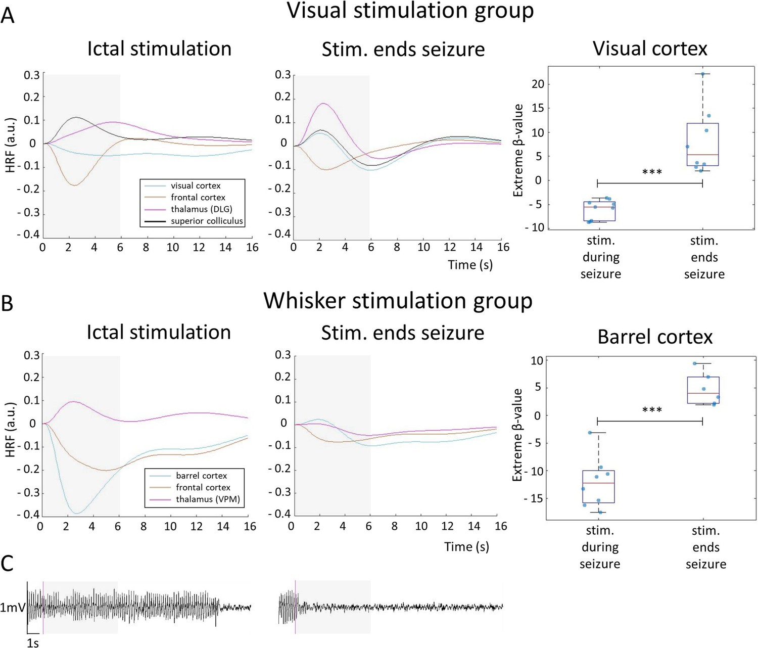
Hemodynamic response functions (HRFs) to stimulation during an ictal period and during a condition when stimulation ended a seizure, for visual stimulation (A) and whisker stimulation (B) groups.
HRF was calculated in selected ROI, belonging to visual or somatosensory area, by multiplying gamma basis functions (Figure 1—figure supplement 1B) with their corresponding average beta-values over a ROI and taking a sum of these values. For statistical comparison, extreme beta-values over a ROI were calculated and values between two states were compared with a two-sample t-test (n=9 sesions in visual stimulation group, n=8 in whisker stimulation group). Scatter plots represent mean ± SD and each blue dot corresponds to the extreme beta-values observed during individual functional magnetic resonance imaging (fMRI) sessions. A representative period from EEG trace, with a stimulation onset marked (purple), in both conditions is also illustrated (C). ***=p<0.001. Gray box illustrates stimulation period.
Figure 5
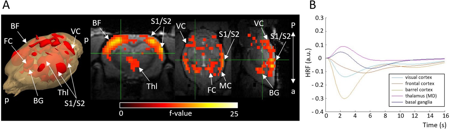
Activation F-contrast map (A) and hemodynamic response functions (HRFs) to seizure (B).
Parameter estimates of regressors were calculated for every voxel, and contrasts were added to parameter estimates of seizure in absence of stimulation. For statistical significance, F-contrast (p<0.05) maps were created and corrected for multiple comparisons by cluster-level correction. HRF was calculated in selected ROI by multiplying gamma basis functions (Figure 1—figure supplement 1B) with their corresponding average beta-values over a ROI and taking a sum of these values. For both the maps and HRFs, data from visual and whisker stimulation experiments were pooled together. BF = barrel field, BG = basal ganglia, FC = frontal cortex, MD = mediodorsal thalamic nucleus, VC = visual cortex. a = anterior, p = posterior.
Figure 6 with 2 supplements
Simulation of sensory stimulation during ictal and interictal periods.
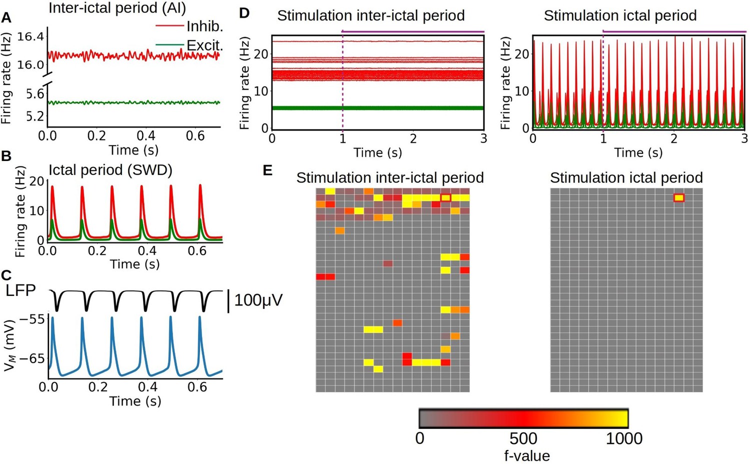
(A–B) Asynchronous irregular (AI) and spike-and-wave discharge (SWD) type of dynamics obtained from the mean-field model, representing interictal and ictal periods respectively. The change between the two dynamics is given by the strength of the adaptation current in the adaptive exponential LIF neurons (AdEx) mean-field model. (C) Local field potential (LFP) and membrane potential obtained from the mean-field model. The model can capture the SWD pattern observed experimentally in LFP measurements which is correlated with periods of hyper-polarization in the membrane potential. (D–E) Time-series and statistical maps of the simulated sensory stimulus in the whole-brain simulations of the rat, showing the results of a stimulation of the primary visual cortex during ictal and interictal periods. The onset and duration of the stimulus is indicated by the dashed vertical line and horizontal line at the top of the time-series. The statistical maps are built from a 2D representation of the 496 brain regions of the BAMS rat connectome described in the method section "Modeling and simulations".
Figure 6—figure supplement 1

Single region activity during stimulation in whole-brain simulation.
We show the results of the simulations during interictal (A, B, C) and ictal periods (D, E, F). The stimulus is applied in the primary visual cortex (A, D) and propagates to the connected regions. In panels B, C, E, and F we show the excitatory (green) and inhibitory (red) activity in the mediolateral visual area during interictal (B, C) and ictal (E, F) periods. For a better visualization the rolling average is shown in dark green and dark red respectively.
Figure 6—figure supplement 2
Comparison of the spike-and-wave discharge (SWD) dynamics in the mean-field model and a spiking-neural network of adaptive exponential LIF neurons (AdEx) neurons.
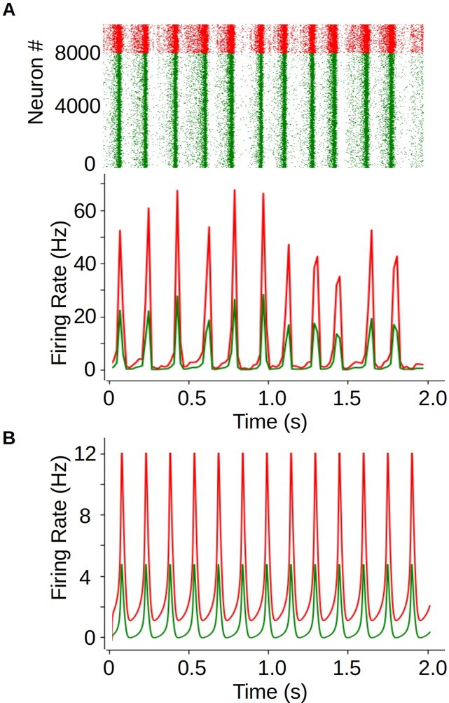
(A) Raster plot (top) and mean firing rate (bottom) from an SWD type of dynamics obtained from the spiking network simulations. The network is made of 8000 excitatory neurons and 2000 inhibitory neurons. Neurons in the network are randomly connected with a probability p=0.05 for inhibitory-inhibitory and excitatory-inhibitory connections, and p=0.06 for excitatory-excitatory connections. Cellular parameters correspond to the ones used in the mean-field, with spike-triggered adaptation for excitatory neurons set to b=200 pA. We show the results for excitatory (green) and inhibitory (red) neurons. (B) Mean firing rate obtained from a single mean-field model. We see that, although the amplitude of oscillations is larger in the spiking network, the mean-field can correctly capture the general dynamics and frequency of the oscillations.
Tables
Table 1
Characteristics of the stimulations and seizures during a 45 min functional magnetic resonance imaging (fMRI) scanning period.
Occurrences (numbers/45 min) of each stimulation type during scanning period are presented, as well as occurrences and duration of seizures.
| Visual stimulation group | Whisker stimulation group | ||||
|---|---|---|---|---|---|
| Stimulations (nr/45 min) | Stimulations (nr/45 min) | ||||
| Mean | SD | Mean | SD | ||
| Stimulation during baseline | 32.4 | 12.3 | Stimulation during baseline | 22.2 | 8.8 |
| Stimulation fully inside seizure | 11.4 | 8.2 | Stimulation fully inside seizure | 9.9 | 9.5 |
| Stimulation started during seizure, >50% inside of seizure | 2.9 | 3.0 | Stimulation started during seizure, >50% inside of seizure | 2.1 | 2.2 |
| Stimulation started during seizure, >50% outside of seizure | 3.9 | 2.5 | Stimulation started during seizure, >50% outside of seizure | 3.5 | 4.0 |
| Stimulation started before seizure, >50% inside of seizure | 1.5 | 1.6 | Stimulation started before seizure, >50% inside of seizure | 0.1 | 0.3 |
| Stimulation started before seizure, >50% outside of seizure | 1.3 | 1.5 | Stimulation started before seizure, >50% outside of seizure | 0.5 | 0.8 |
| Stimulation ended seizure | 3.1 | 2.8 | Stimulation ended seizure | 12 | 8.1 |
| Stimulation right after seizure | 1.1 | 0.8 | Stimulation right after seizure | 1.8 | 1.6 |
| Seizures | Seizures | ||||
| Total number of seizures | 40.2 | 28.3 | Total number of seizures | 49.6 | 34.6 |
| Seizures without a stimulation | 15 | 7.8 | Seizures without a stimulation | 19.8 | 8.2 |
| Duration of seizures (s) | 6.1 | 5.2 | Duration of seizures (s) | 5.1 | 4.0 |
Additional files
Download links
A two-part list of links to download the article, or parts of the article, in various formats.
Downloads (link to download the article as PDF)
Open citations (links to open the citations from this article in various online reference manager services)
Cite this article (links to download the citations from this article in formats compatible with various reference manager tools)
EEG-fMRI in awake rat and whole-brain simulations show decreased brain responsiveness to sensory stimulations during absence seizures
eLife 12:RP90318.
https://doi.org/10.7554/eLife.90318.4


