A neural correlate of individual odor preference in Drosophila
- Organismic and Evolutionary Biology, Harvard University, United States
- Center for Brain Science, Harvard University, Cambridge, United States
- McGovern Institute, MIT, United States
- MIT Media Lab, MIT, United States
- Janelia Research Campus, Howard Hughes Medical Institute, United States
- Department of Biological Engineering, MIT, United States
- Koch Institute, Department of Biology, MIT, United States
- Howard Hughes Medical Institute, United States
- Department of Brain and Cognitive Sciences, MIT, United States
Figures
Figure 1 with 10 supplements
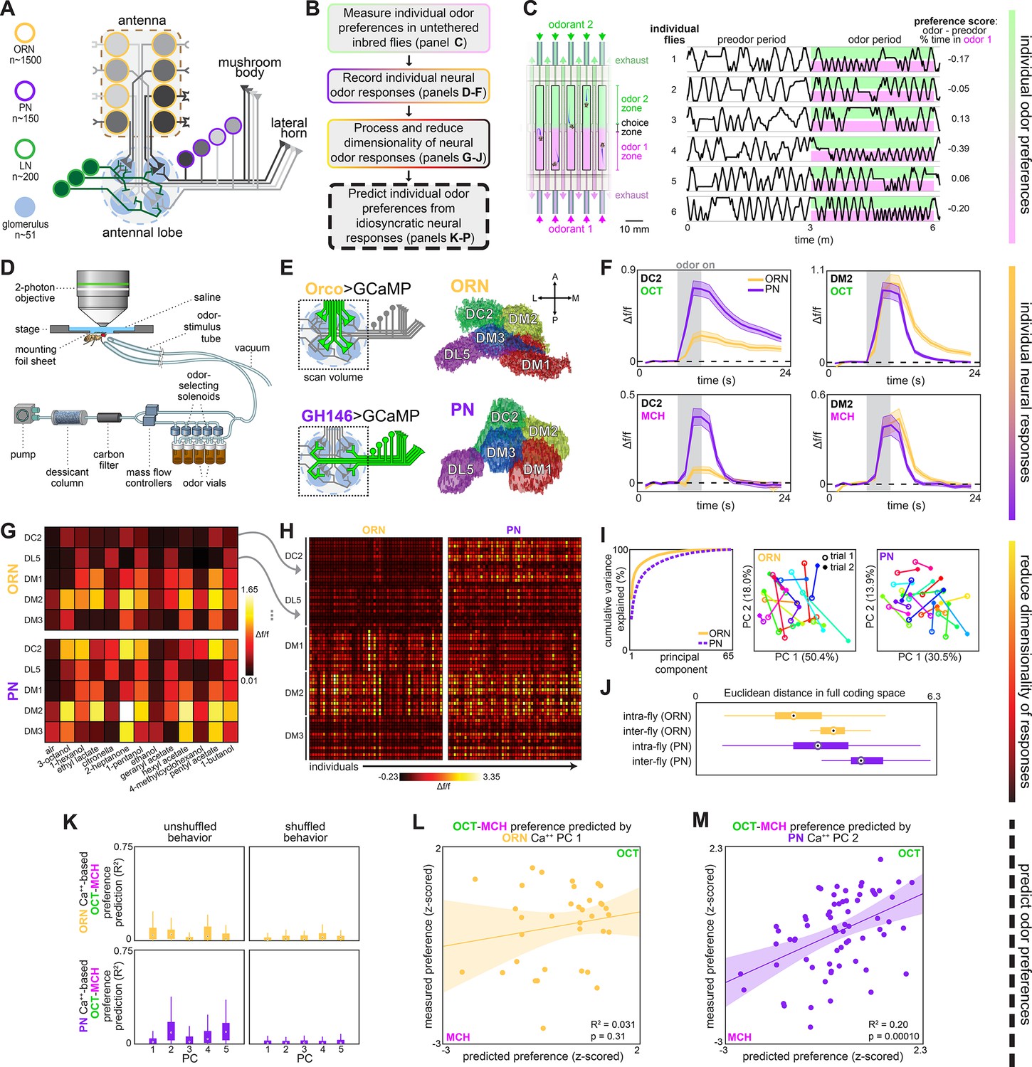
Idiosyncratic calcium dynamics predict individual odor preferences.
(A) Olfactory circuit schematic. Olfactory receptor neurons (ORNs, peach outline) and projection neurons (PNs, plum outline) are comprised of ~51 classes corresponding to odor receptor response channels. ORNs (gray shading) sense odors in the antennae and synapse on dendrites of PNs of the same class in ball-shaped structures called glomeruli located in the antennal lobe (AL). Local neurons (LNs, green outline) mediate interglomerular cross-talk and presynaptic inhibition, amongst other roles (Olsen and Wilson, 2008; Yaksi and Wilson, 2010). Odor signals are normalized and whitened in the AL before being sent to the mushroom body and lateral horn for further processing. Schematic adapted from Figure 2C of Honegger et al., 2020. (B) Experiment outline. (C) Odor preference behavior tracking setup (reproduced from Figure 1B of Honegger et al., 2020) and example individual fly ethograms. OCT (green) and MCH (magenta) were presented for 3 minutes. (D) Head-fixed two-photon calcium imaging and odor delivery setup (reproduced from Figure 2A of Honegger et al., 2020). (E) Orco and GH146 driver expression profiles (left) and example segmentation masks (right) extracted from two-photon calcium images for a single fly expressing Orco>GCaMP6m (top, expressed in a subset of all ORN classes) or GH146>GCaMP6m (bottom, expressed in a subset of all PN classes). (F) Time-dependent Δf/f for glomerular odor responses in ORNs (peach) and PNs (plum) averaged across all individuals: DC2 to OCT (upper left), DM2 to OCT (upper right), DC2 to MCH (lower left), and DM2 to OCT (lower right). Shaded error bars represent S.E.M. (G) Peak Δf/f for each glomerulus-odor pair averaged across all flies. (H) Individual neural responses measured in ORNs (left) or PNs (right) for 50 flies each. Columns represent the average of up to four odor responses from a single fly. Each row represents one glomerulus-odor response pair. Odors are the same as in panel (G). (I) Principal component analysis of individual neural responses. Fraction of variance explained vs. principal component number (left). Trial 1 and trial 2 of ORN (middle) and PN (right) responses for 20 individuals (unique colors) embedded in PC 1–2 space. (J) Euclidean distances between glomerulus-odor responses within and across flies measured in ORNs (n = 65 flies) and PNs (n = 122 flies). Distances calculated without PCA compression. (K) Bootstrapped R2 of OCT-MCH preference prediction from each of the first five principal components of neural activity measured in ORNs (top, all data) or PNs (bottom, training set). (L) Measured OCT-MCH preference vs. preference predicted from PC 1 of ORN activity (n = 35 flies). (M) Measured OCT-MCH preference vs. preference predicted from PC 2 of PN activity in n = 69 flies using a model trained on a training set of n = 47 flies (see Figure 2—figure supplement 1C and D for train/test flies analyzed separately). Shaded regions in (L, M) are the 95% CIs of the fit estimated by bootstrapping. In (J, K), points represent the median value, boxes represent the interquartile range, and whiskers the range of the data.
Figure 1—figure supplement 1
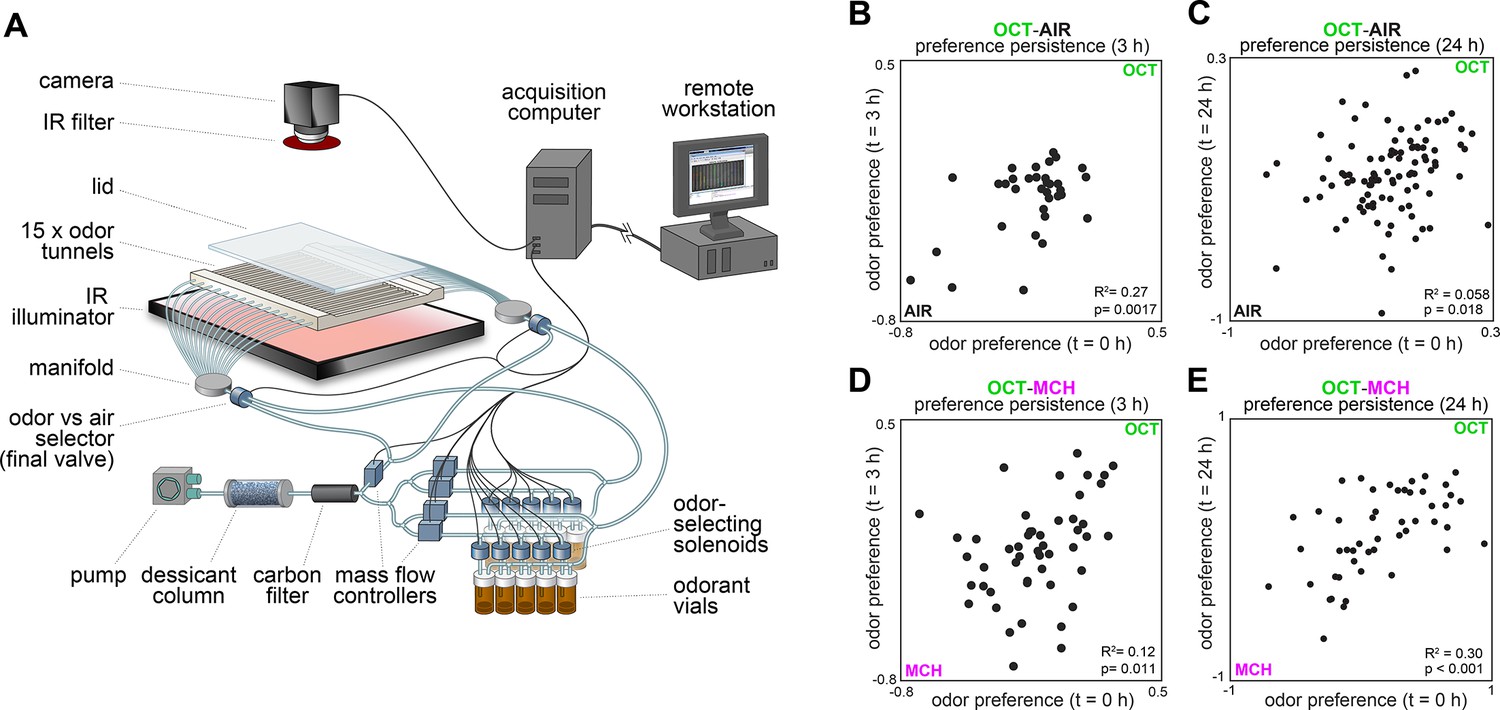
Behavioral measurements and individual preference persistence.
(A) Behavioral measurement apparatus (adapted from Figure 1A of Honegger et al., 2020). (B) Odor preference persistence over 3 hours for flies given a choice between 3-octanol and air (n = 34 flies). (C) Odor preference persistence over 24 hours for flies given a choice between 3-octanol and air (n = 97 flies). (D) Odor preference persistence over 3 hours for flies given a choice between 3-octanol and 4-methylcyclohexanol (n = 51 flies). (E) Odor preference persistence over 24 hours for flies given a choice between 3-octanol and 4-methylcyclohexanol (n = 49 flies).
Figure 1—figure supplement 2
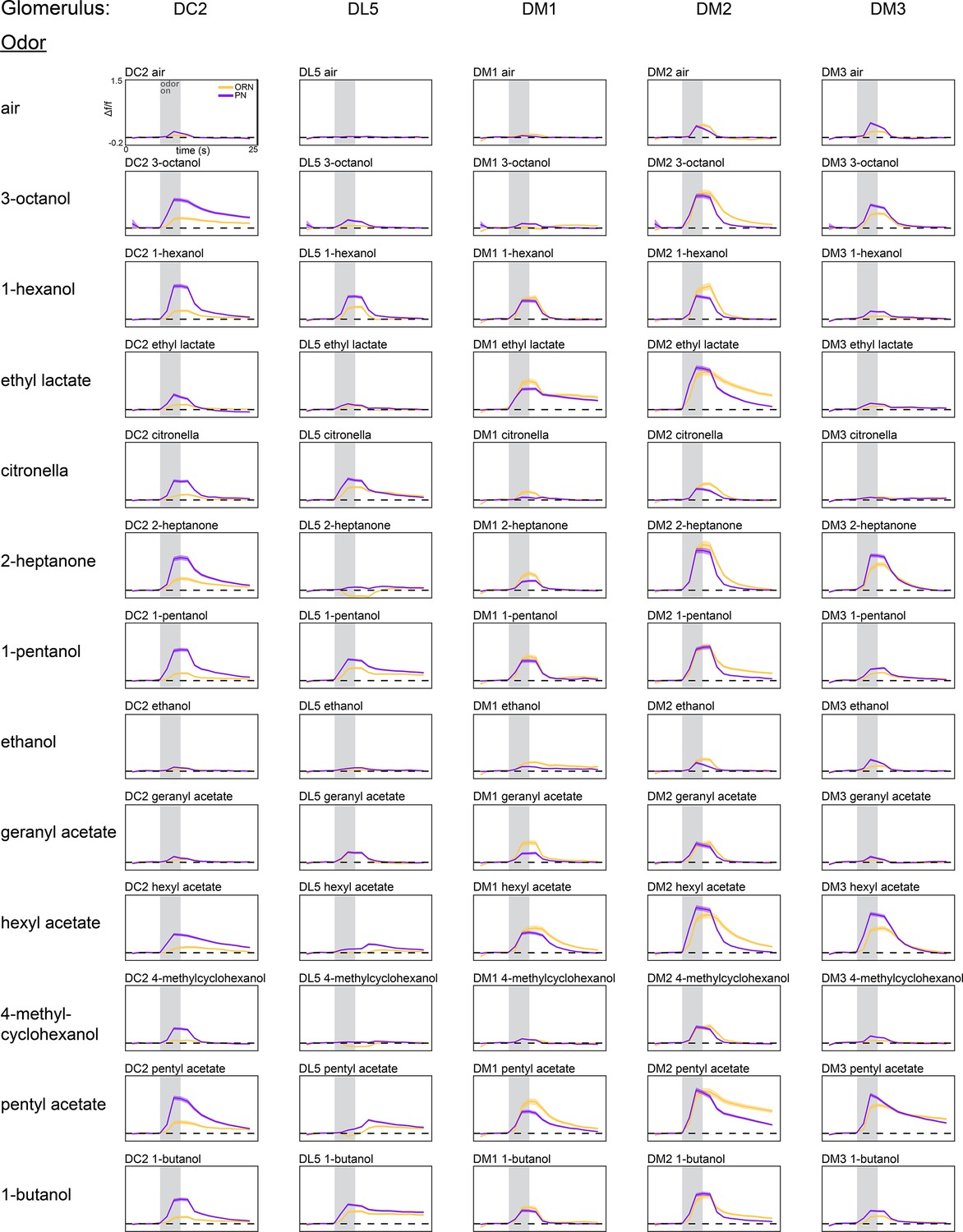
Average glomerulus-odor time-dependent responses.
Time-dependent responses of each glomerulus identified in our study to the 13 odors in our odor panel. Data represents the average across flies (olfactory receptor neuron [ORN], peach curves, n = 65 flies; projection neuron [PN], plum curves, n = 122 flies). Shaded error bars represent S.E.M.
Figure 1—figure supplement 3

Individual glomerulus-odor responses.
Idiosyncratic odor coding measured in olfactory receptor neurons (ORNs) (left, 208 recordings across 65 flies) and projection neurons (PNs) (right, 406 trials across 122 flies). Each column represents the response (max Δf/f attained over the odor trial) in a single recording from either the left or right lobe of a single fly. Below each heatmap, markers are grouped by individual fly (fly order is arbitrary, markers of adjacent flies alternate in height). Green markers correspond to left lobes, blue markers right lobes. Each row represents a glomerulus-odor response pair. Missing data are indicated in gray.
Figure 1—figure supplement 4
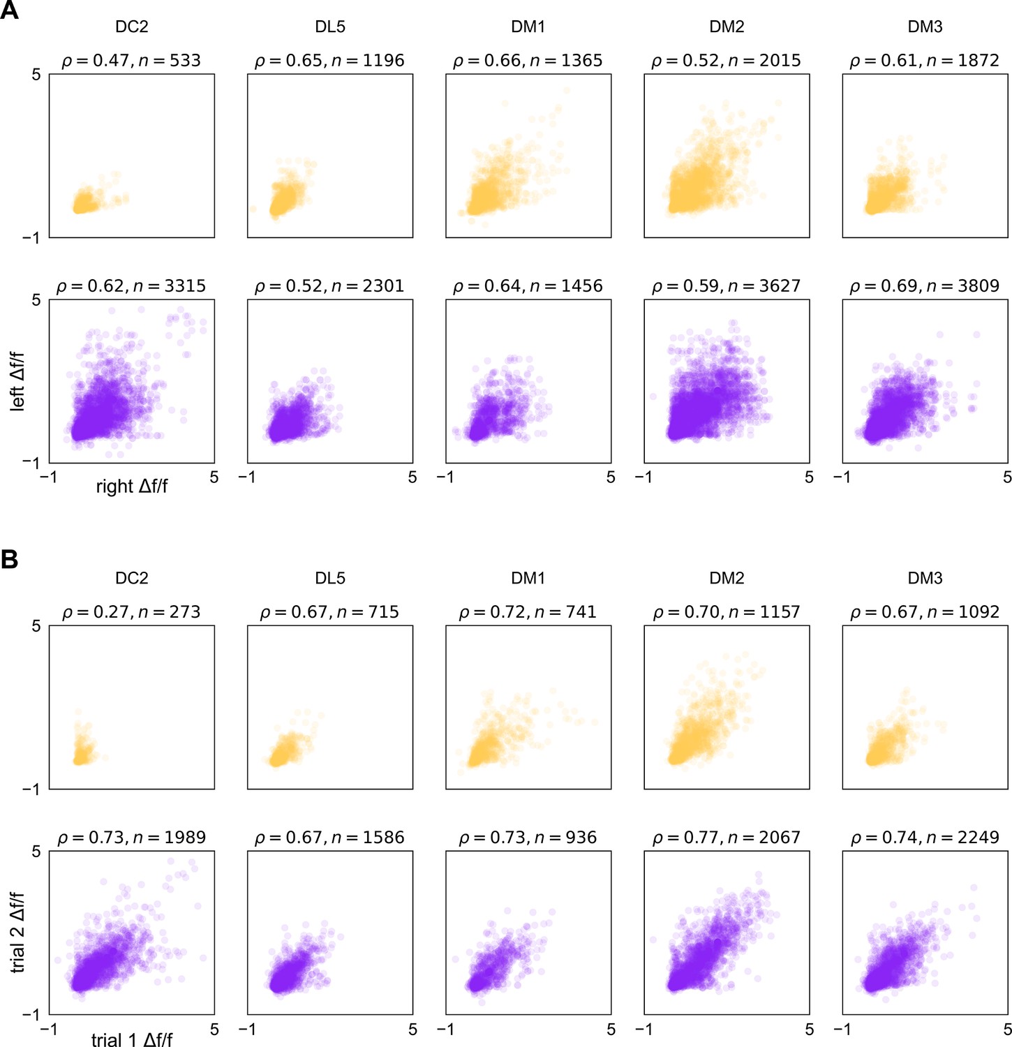
Correspondence in calcium responses between lobes and trials.
(A) Scatter plots of max Δf/f attained over an odor presentation in a left-lobe recording vs. a right-lobe recording in the same fly (same data as presented in Figure 1—figure supplement 3). Plum points are projection neuron (PN) responses and peach points olfactory receptor neurons (ORNs). ρ is Spearman’s rank correlation coefficient, points correspond to fly-odor-trial combinations, and n indicates the number of points within each subplot. (B) As in (A), for responses across two trials within the same lobe of the same fly. Points correspond to fly-odor-lobe combinations.
Figure 1—figure supplement 5
Glomerulus responses and identification.
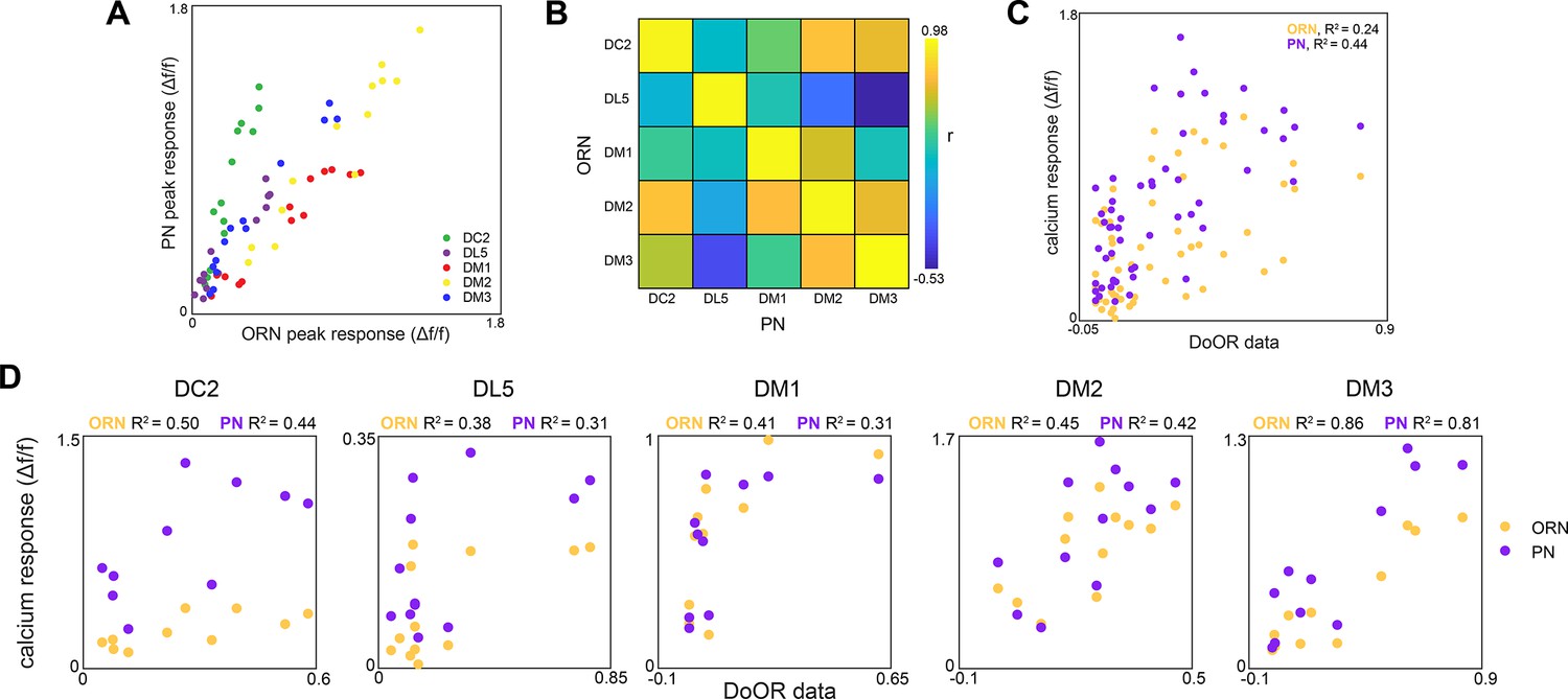
(A) Glomerulus odor responses measured in projection neurons (PNs) vs. those measured in olfactory receptor neurons (ORNs) (n = 65 flies). Points correspond to the odorants listed in Figure 1G. (B) Cross-odor trial correlation matrix between glomerular odor responses in ORNs and PNs. (C) Peak calcium responses for each glomerulus-odor pair measured in this study plotted against those recorded in the DoOR dataset (Münch and Galizia, 2016). (D) Peak calcium responses for each individual glomerulus plotted against those recorded in the DoOR dataset.
Figure 1—figure supplement 6
Idiosyncrasy of olfactory receptor neuron (ORN) and projection neuron (PN) responses.
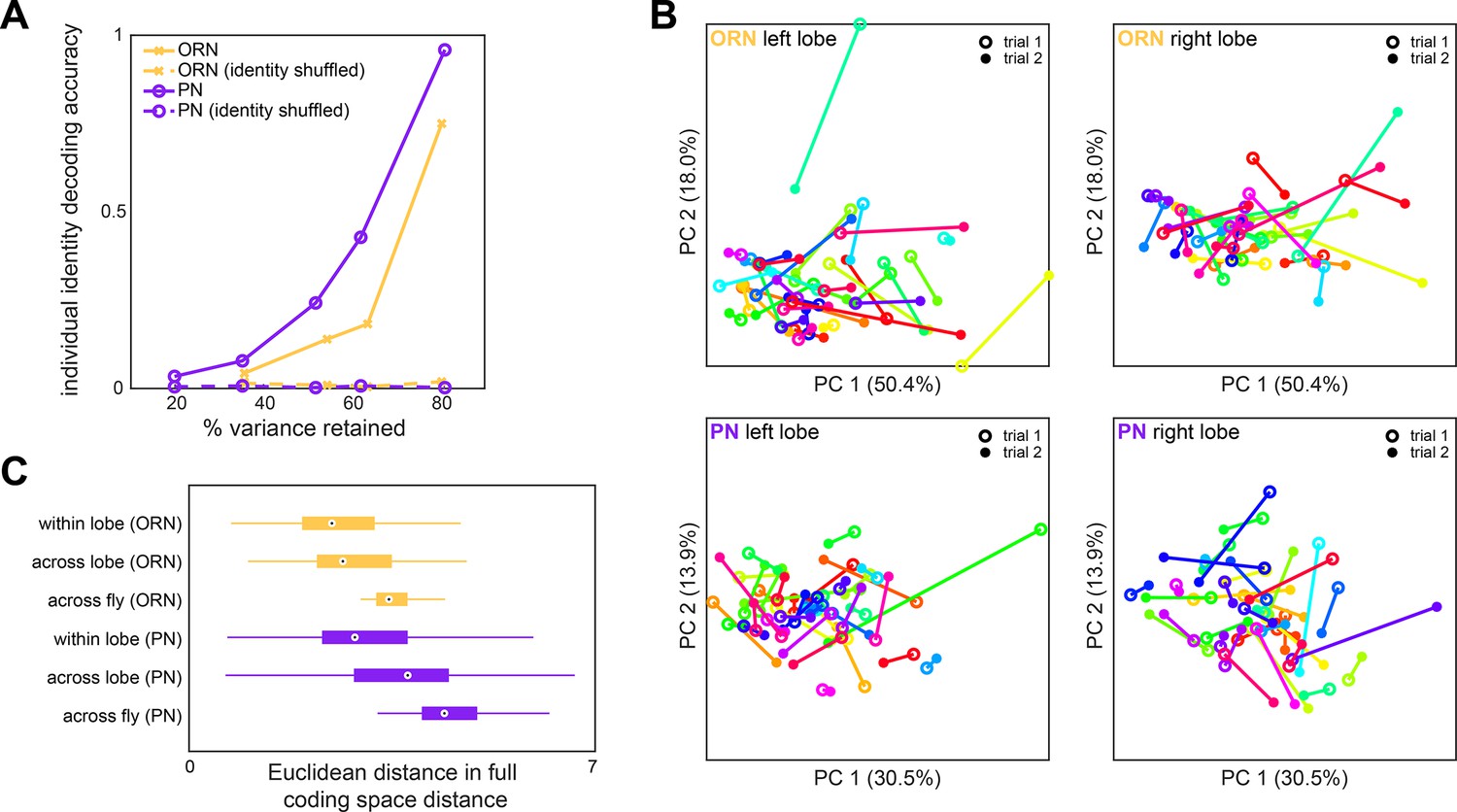
(A) Logistic regression classifier accuracy of decoding individual identity from individual odor panel peak responses. PCA was performed on population responses and the specified fraction of variance (x-axis) was retained. Individual identity can be better decoded from PN responses (n = 122 flies) than ORN responses (n = 65 flies) in all cases. (B) Individual trial-to-trial glomerulus-odor responses embedded in PC 1–2 space. Responses for the same flies as Figure 1I are shown. Each linked color represents one fly. Trial 1 and trial 2 responses are shown for ORN left lobe (upper left), ORN right lobe (upper right), PN left lobe (lower left), and PN right lobe (lower right). (C) Distance in the full glomerulus-odor response space between recordings within a lobe (trial-to-trial), across lobes (within fly), and across flies for ORNs and PNs. Points represent the median value, boxes represent the interquartile range, and whiskers the range of the data.
Figure 1—figure supplement 7
Calcium response correlation matrices.
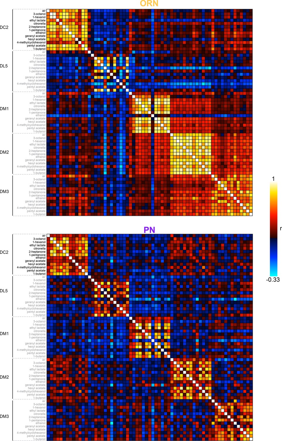
Correlation between calcium response dimensions across flies measured in olfactory receptor neurons (ORNs, n = 65 flies) (top) and projection neurons (PNs, n = 122 flies) (bottom). Glomerulus-odor responses are correlated at the level of glomeruli in both cell types. Inter-glomerulus correlations are more prominent in ORNs than PNs, consistent with known antennal lobe (AL) transformations that result in decorrelated PN activity (Bhandawat et al., 2007; Luo et al., 2010).
Figure 1—figure supplement 8
Calcium imaging principal component loadings.
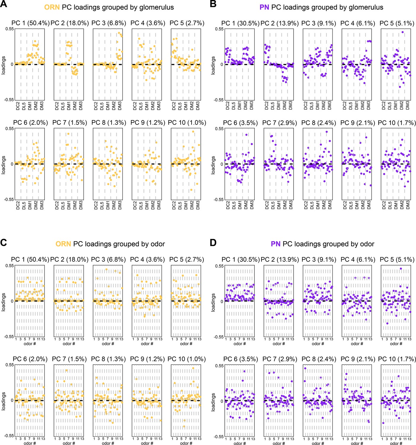
(A, B) First 10 principal component loadings measured from calcium responses in olfactory receptor neurons (ORNs) (A, n = 65 flies) and projection neurons (PNs) (B, n = 122 flies). Loadings are grouped by glomerulus, with each loading within a glomerulus representing the response of that glomerulus to one odor in the odor panel. Odors are the same as those listed in Figure 1G. (C, D) The same 10 principal component loadings as those shown in panels (A, B) grouped by odor rather than glomerulus. Glomeruli within each odor block are given in the order of panels (A) and (B).
Figure 1—figure supplement 9
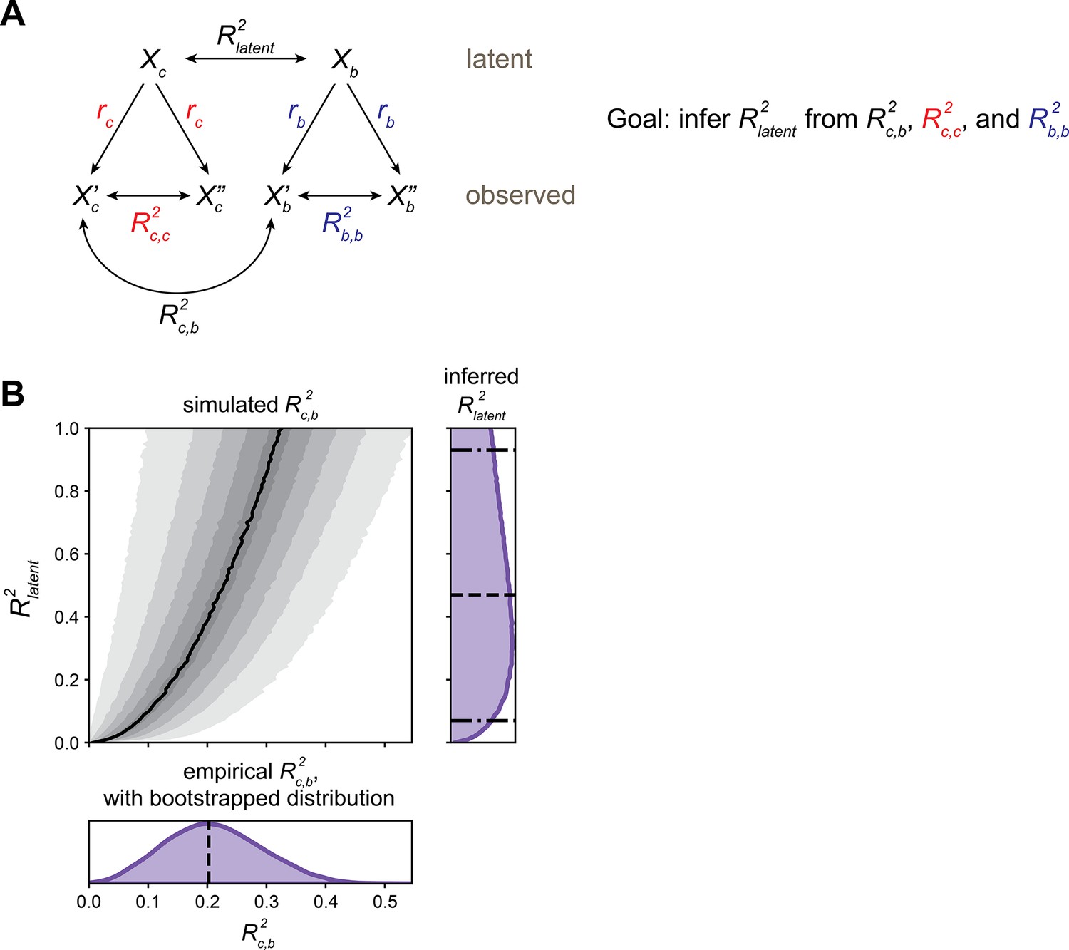
Estimating latent calcium–behavior correlations.
(A) Schematic of inference approach to estimate the correlation between latent calcium (c) and behavioral (b) states (R2latent). This method can be applied identically to infer R2latent between Brp measurements and behavior. (B) Demonstration of R2latent inference for olfactory receptor neuron (ORN) vs. 4-methylcyclohexanol (MCH) model presented in Figure 1M: Projection neuron (PN) calcium PC 2 from trained model applied to train+test data. Bottom subplot: bootstrap distribution of calcium–behavior R2c,b (dashed line: R2c,b = 0.20 for the N = 69 flies). Top left subplot: simulated R2c,b values. Black line indicates median R2c,b among the 10,000 simulations for each R2latent, shaded areas (from lightest to darkest to lightest) indicate 5–15th, 15–25th, …, 85–95th percentile R2c,b. Right subplot: inferred distribution for R2latent, estimated by adding marginal distributions over R2latent for R2c,b values sampled from the bootstrap R2c,b distribution. The median R2latent is 0.46 (dashed line), with 90% CI 0.06–0.90 estimated by the 5th–95th percentiles of the marginal distribution (dot-dashed lines).
Figure 1—figure supplement 10
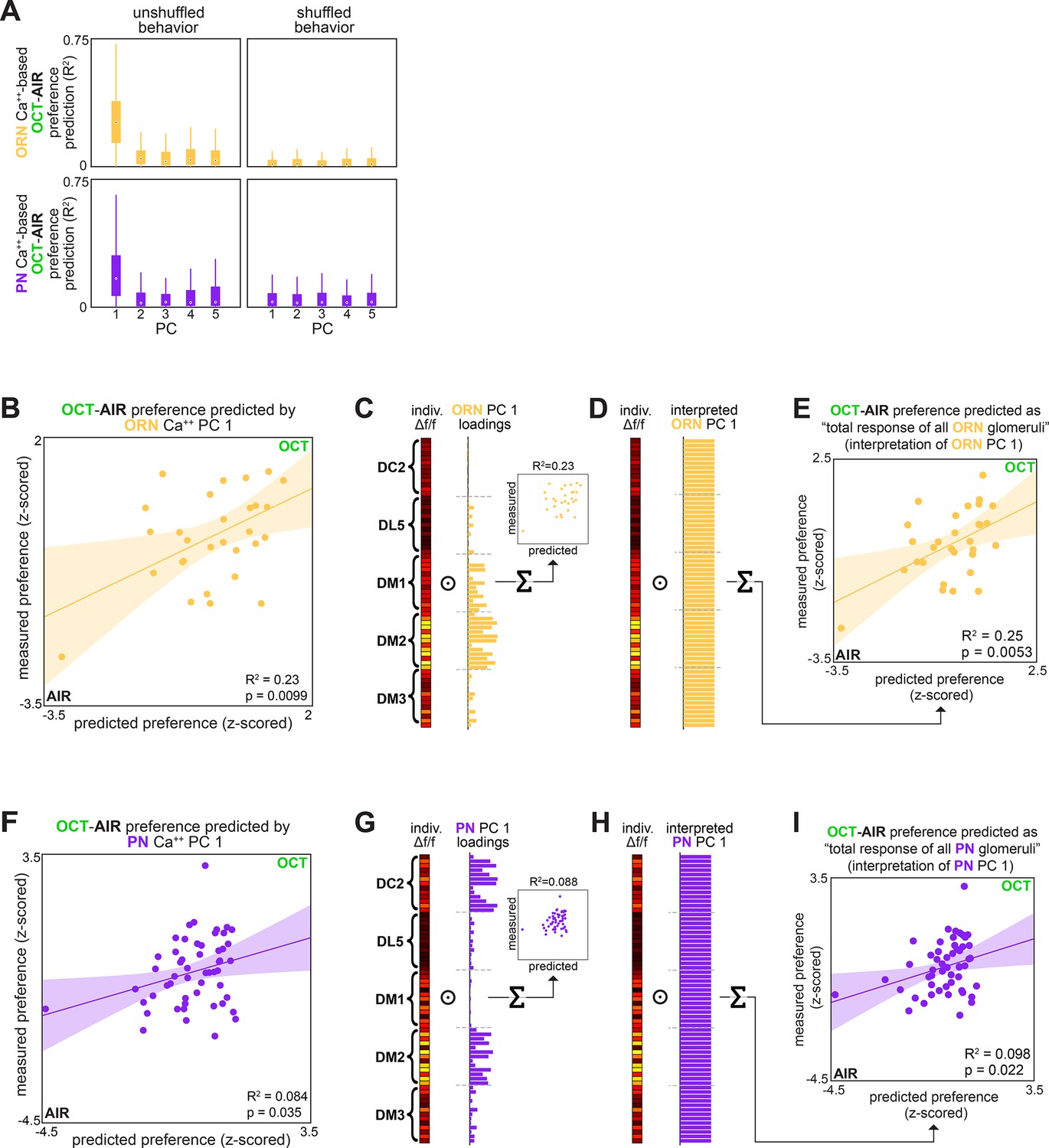
OCT-AIR preference prediction.
(A) Bootstrapped R2 of OCT-AIR preference prediction from each of the first five principal components of neural activity measured in olfactory receptor neurons (ORNs) (top, all data) or projection neurons (PNs) (bottom, training set). Points represent the median value, boxes represent the interquartile range, and whiskers the range of the data. (B) Measured OCT-AIR preference vs. preference predicted from PC 1 of ORN activity (n = 30 flies). (C) PC 1 loadings of ORN activity for flies in (B). (D) Interpreted ORN PC 1 loadings. (E) Measured OCT-AIR preference vs. preference predicted by the average peak response across all ORN coding dimensions (n = 30 flies). (F) Measured OCT-AIR preference vs. preference predicted from PC 1 of PN activity in n = 53 flies using a model trained on a training set of n = 18 flies (see Figure 2—figure supplement 1A and B for train/test flies analyzed separately). (G) PC 2 loadings of PN activity for flies in (F). (H) Interpreted PN PC2 loadings. (I) Measured OCT-MCH preference vs. preference predicted by the average peak PN response in DM2 minus DC2 across all odors (n = 69 flies).
Figure 2 with 2 supplements
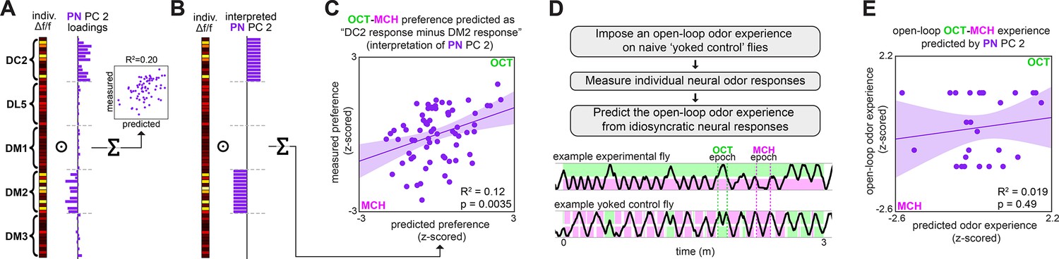
Variation in relative glomerular responses explains individual odor preference.
(A) PC 2 loadings of projection neuron (PN) activity for flies tested for OCT-MCH preference (n = 69 flies). (B) Interpreted PN PC 2 loadings. (C) Measured OCT-MCH preference vs. preference predicted by the average peak PN response in DM2 minus DC2 across all odors (n = 69 flies). (D) Yoked-control experiment outline and example behavior traces. Experimental flies are free to move about tunnels permeated with steady-state OCT and MCH flowing into either end. Yoked-control flies are delivered the same odor at both ends of the tunnel that matches the odor experienced at the nose of the experimental fly at each moment in time. (E) Imposed odor experience vs. the odor experience predicted from PC 2 of PN activity (n = 27 flies) evaluated on the model trained from data in Figure 1M. Shaded regions in (C, E) are the 95% CIs of the fit estimated by bootstrapping.
Figure 2—figure supplement 1

Measured preference vs. projection neuron (PN) activity-based predicted preference, split by training/testing set.
(A) Measured OCT-AIR preference vs. preference predicted from PC 1 of PN activity in a training set (n = 18 flies). (B) Measured OCT-AIR preference vs. preference predicted from PC 1 on PN activity in a test set (n = 35 flies) evaluated on a model trained on data from panel (A). (C) Measured OCT-MCH preference vs. preference predicted from PC 2 of PN activity in a training set (n = 47 flies). (D) Measured OCT-MCH preference vs. preference predicted from PC 2 on PN activity in a test set (n = 22 flies) evaluated on a model trained on data from panel (C).
Figure 2—figure supplement 2
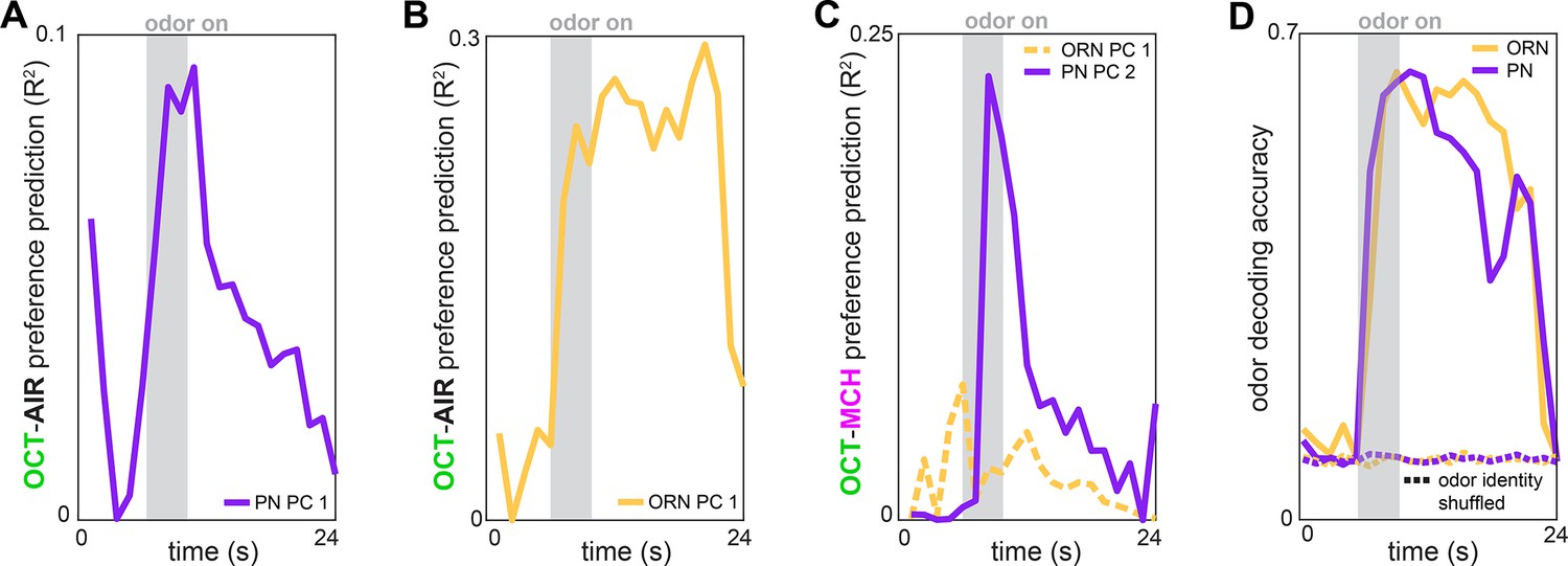
Time-dependent preference- and odor-decoding.
(A) R2 of odor-vs.-air preference predicted by PC 1 of projection neuron (PN) activity as a function of time across trials (n = 53 flies). (B) R2 of odor-vs.-air preference predicted by PC 1 of olfactory receptor neuron (ORN) activity as a function of time across trials (n = 30 flies). (C) R2 of odor-vs.-odor preference predicted by PC 2 of PN activity (solid plum, n = 69 flies) or PC 1 of ORN activity (dashed peach, n = 35 flies) as a function of time across trials. (D) Logistic regression classifier accuracy of decoding odor identity from 5 glomerular responses as a function of time. Dashed curves indicate performance on shuffled data.
Figure 3 with 2 supplements
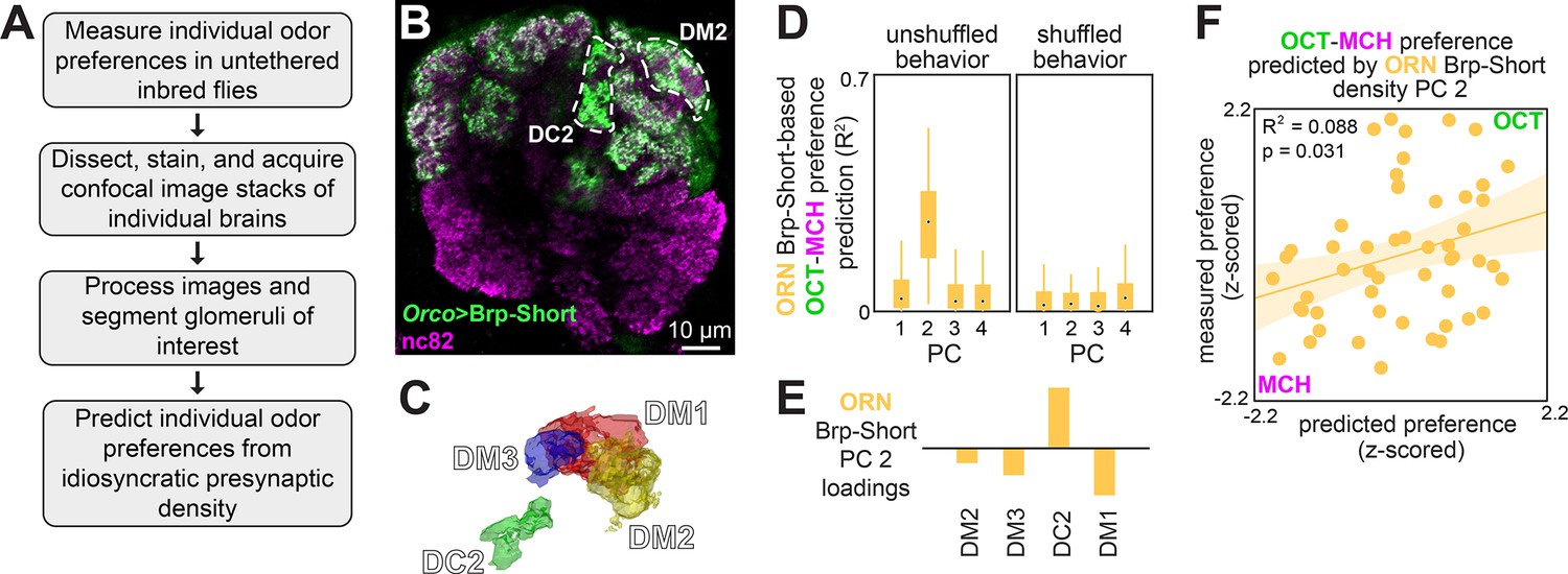
Idiosyncratic presynaptic marker density in DM2 and DC2 predicts OCT-MCH preference.
(A) Experiment outline. (B) Example slice from a z-stack of the antennal lobe expressing Orco>Brp-Short (green) with DC2 and DM2 visible (white dashed outline). nc82 counterstain (magenta). (C) Example glomerulus segmentation masks extracted from an individual z-stack. (D) Bootstrapped R2 of OCT-MCH preference prediction from each of the first four principal components of Brp-Short density measured in olfactory receptor neurons (ORNs) (training set, n = 22 flies). Points represent the median value, boxes represent the interquartile range, and whiskers the range of the data. (E) PC 2 loadings of Brp-Short density. (F) Measured OCT-MCH preference vs. preference predicted from PC 2 of ORN Brp-Short density in n = 53 flies using a model trained on a training set of n = 22 flies (see Figure 3—figure supplement 1 for train/test flies analyzed separately).
Figure 3—figure supplement 1
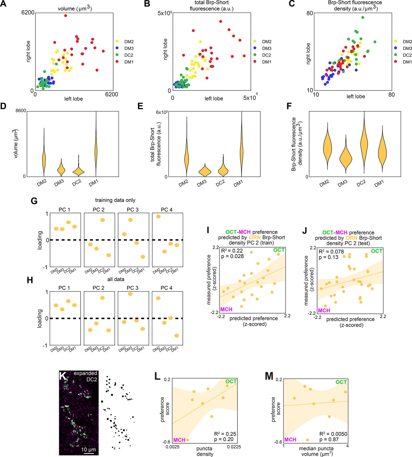
ORN>Brp-Short characterization and model predictions.
(A–C) Right vs. left glomerulus properties measured from z-stacks of stained Orco>Brp-Short samples from a training set of flies (n = 22): (A) Volume, (B) total Brp-Short fluorescence, and (C) Brp-Short fluorescence density. (D–F) Same data as panels (A–C) represented in violin plots (kernel density estimated). (G) Principal component loadings of Brp-Short density calculated using only training data (n = 22 flies). (H) Principal component loadings of Brp-Short density calculated using all data (n = 53 flies). (I) Measured OCT-MCH preference vs. preference predicted from PC 2 of ORN Brp-Short density in a training set (n = 22 flies). (J) Measured OCT-MCH preference vs. preference predicted from PC 2 on ORN Brp-Short density in a test set (n = 31 flies) evaluated on a model trained on data from panel (I). (K) Example expanded antennal lobe (AL) expressing Or13a>Brp-Short (left) and Imaris-identified puncta from that sample (right). (L) OCT-MCH preference score plotted against Brp-Short puncta density in expanded Or13a>Brp-Short samples (n = 8 flies). (M) OCT-MCH preference score plotted against Brp-Short median puncta volume in expanded Or13a>Brp-Short samples (n = 8 flies). Shaded regions in (I, J, L, M) are the 95%CI of the fit estimated by bootstrapping.
Figure 3—figure supplement 2
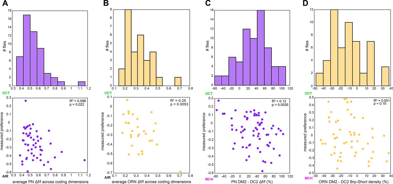
Calcium and Brp-Short predictor variation.
(A) Histogram of average projection neuron (PN) Δf/f across all coding dimensions in flies in which OCT-AIR preference was measured (top) and OCT-AIR preference vs. average PN Δf/f (n = 53 flies) (bottom). (B) Similar to (A) for ORN Δf/f and OCT-AIR preference (n = 30 flies). (C) Similar to (A) for Δf/f difference between DM2 and DC2 PN responses and OCT-MCH preference (n = 69 flies). (D) Similar to (A) for % Brp-Short density difference between DM2 and DC2 ORNs and OCT-MCH (n = 53 flies).
Figure 4 with 6 supplements
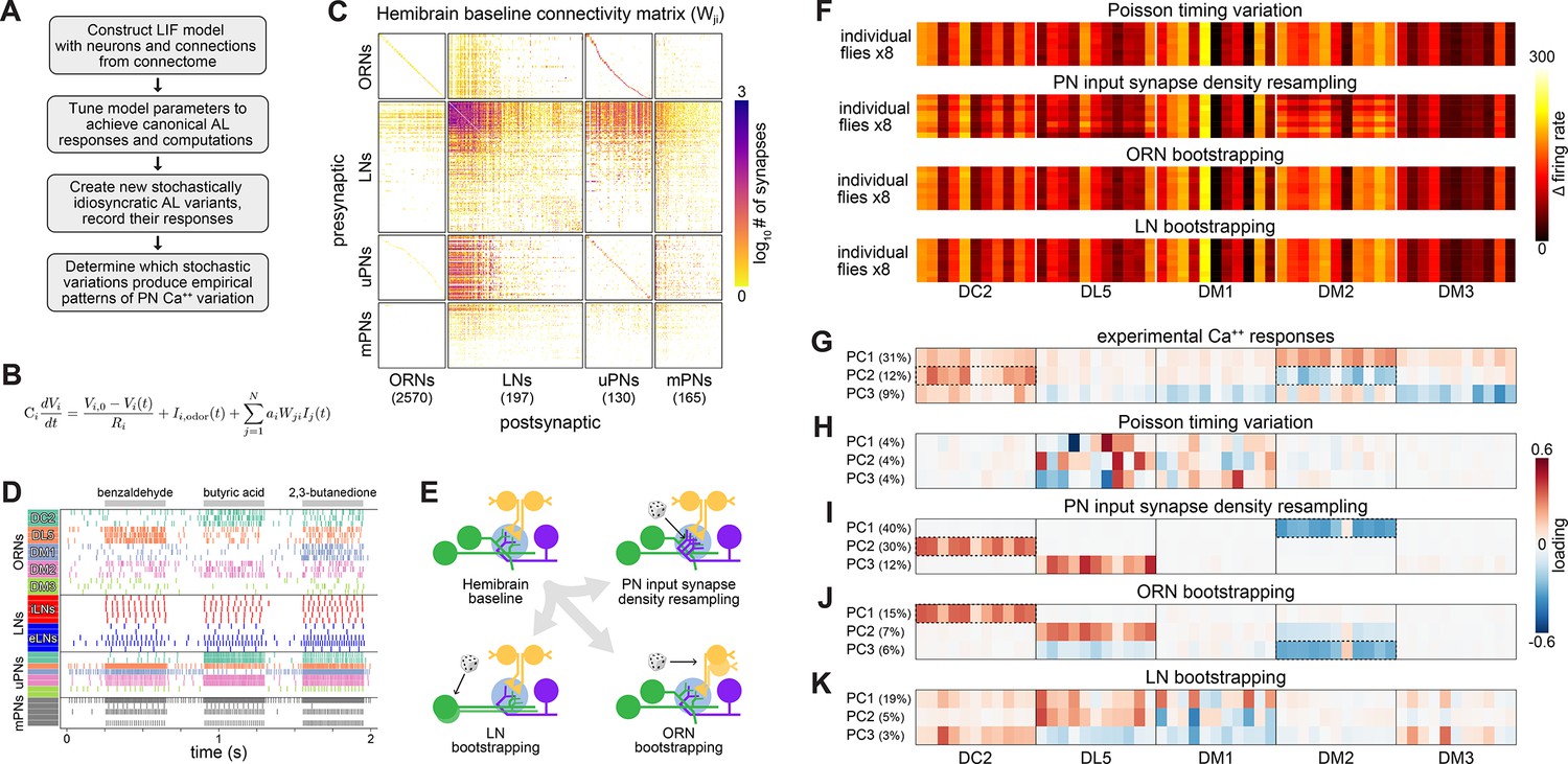
Simulation of olfactory circuits under developmental stochasticity.
(A) Antennal lobe (AL) modeling analysis outline. (B) Leaky-integrator dynamics of each simulated neuron. When a neuron’s voltage reaches its firing threshold, a templated action potential is inserted, and downstream neurons receive a postsynaptic current. See ‘Antennal lobe modeling’ in ‘Materials and methods’. (C) Synaptic weight connectivity matrix, derived from the hemibrain connectome (Scheffer et al., 2020). (D) Spike raster for randomly selected example neurons from each AL cell type. Colors indicate olfactory receptor neuron (ORN)/projection neuron (PN) glomerular identity and LN polarity (i = inhibitory, e = excitatory). (E) Schematic illustrating sources of developmental stochasticity as implemented in the simulated AL framework. See Video 4 for the effects of these resampling methods on the synaptic weight connectivity matrix. (F) PN glomerulus-odor response vectors for eight idiosyncratic ALs subject to Input spike Poisson timing variation, PN input synapse density resampling, and ORN and LN population bootstrapping. (G) Loadings of the principal components of PN glomerulus-odor responses as observed across experimental flies (top). Dotted outlines highlight loadings selective for the DC2 and DM2 glomerular responses, which underlie predictions of individual behavioral preference. (H–K) As in (G) for simulated PN glomerulus-odor responses subject to Input spike Poisson timing variation, PN input synapse density resampling, and ORN and LN population bootstrapping. See Figure 4—figure supplement 5 for additional combinations of idiosyncrasy methods. In (F–K) the sequence of odors within each glomerular block is: OCT, 1-hexanol, ethyl-lactate, 2-heptanone, 1-pentanol, ethanol, geranyl acetate, hexyl acetate, MCH, pentyl acetate, and butanol.
Figure 4—figure supplement 1
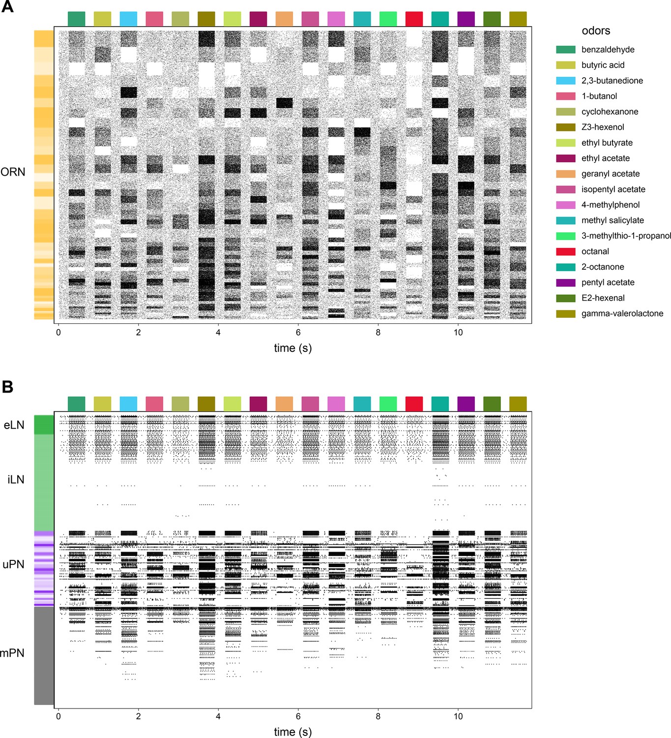
Antennal lobe (AL) model raster plot.
(A) Action potential raster plot of olfactory receptor neurons (ORNs) in the baseline simulated AL. Rows are individual ORNs, black ticks indicate action potentials. Random shades of gold at left indicate blocks of ORN rows projecting to the same glomerulus. (B) The remaining neurons in the model. Shades of green indicate excitatory vs. inhibitory local neurons (LNs) and shades of purple indicate PNs with dendrites in the same glomeruli.
Figure 4—figure supplement 2

Antennal lobe (AL) model baseline outputs compared to experimental data.
(A) Distributions of model neuron firing rates by cell type across odors (transparent black points are individual neuron-odor combinations). Black lozenge symbols indicate the mean firing rate of the points to the right. Yellow stars indicate the comparable experimental values reported in Chou et al., 2010; de Bruyne et al., 2001; Nagel et al., 2015; Wilson et al., 2004. (B) Scatter plots of average projection neuron (PN) firing rate vs. olfactory receptor neuron (ORN) firing rate during odor stimuli in the model vs. experimental values (Bhandawat et al., 2007). Points are odors, colors are glomeruli. (C) Histograms of ON odor minus OFF odor glomerulus-average PN and ORN firing rates in the model vs experimental values (Bhandawat et al., 2007), showing flatter distributions in PNs. (D) Odor representations in the first two PCs of glomerulus-average ORN responses and PN responses in the model and experimental results (Bhandawat et al., 2007). Points are odors. Pairwise distances between PN representations are more uniform than in ORNs in both the model and experimental data. Panels (B–D) use glomerulus-average PN and ORN firing rates from six of the seven glomeruli in Bhandawat et al., 2007, as VM2 is significantly truncated in the hemibrain (Scheffer et al., 2020). Literature features in panels (B–D) were extracted from Bhandawat et al., 2007 using WebPlotDigitizer (Rohatgi, 2021).
Figure 4—figure supplement 3
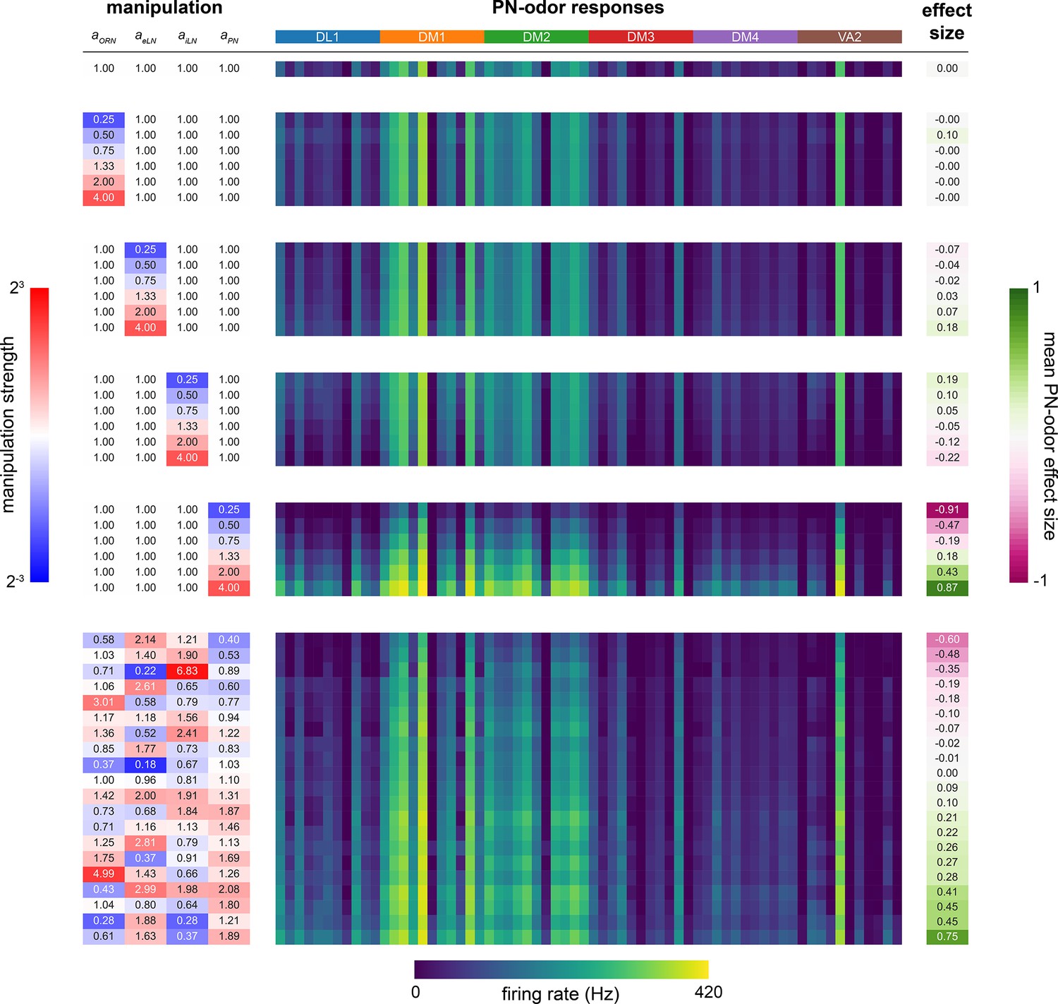
Sensitivity analysis of aORN, aeLN, aiLN, aPN parameters.
Left, blue to red colormap: magnitude of parameter manipulation. Center, dark blue to yellow colormap: mean glomerular firing rate (Hz) responses of projection neurons (PNs) (DL1, DM1, DM2, DM3, DM4, VA2) to 11 odors (order within each glomerulus (colored bands at top): 3-octanol, 1-hexanol, ethyl lactate, 2-heptanone, 1-pentanol, ethanol, geranyl acetate, hexyl acetate, 4-methylcyclohexanol, pentyl acetate, 1-butanol, 3-octanol). Right, pink to green colormap: manipulation effect size on mean PN-odor responses (Cohen’s d). Top: baseline parameter set. Middle: single-parameter manipulations from 1/4× to 4×. Bottom: multiple-parameter manipulations. For further detail, see ‘AL model tuning’ in ‘Materials and methods’. No manipulations yielded effect sizes larger than 0.9; aPN is the most sensitive parameter.
Figure 4—figure supplement 4
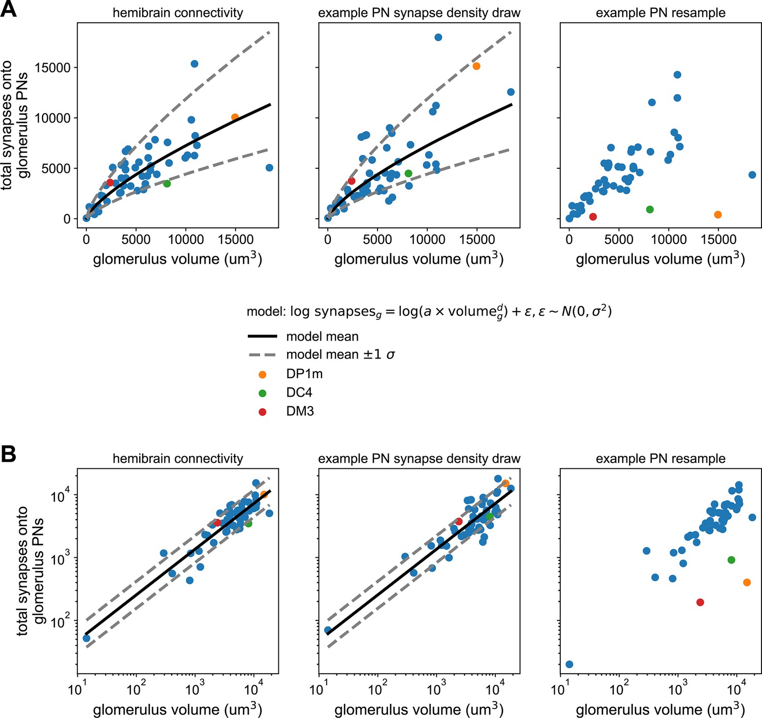
Synapse counts vs. glomerular volume in the hemibrain and antennal lobe (AL) model.
(A) Left: scatter plot of total projection neuron (PN) input synapses within a glomerulus vs. that glomerulus’ volume from the hemibrain dataset. Solid line represents the maximum likelihood-fit mean synapse count vs. glomerular volume, and dashed lines the fit ±1 SD. Middle: As (left) but for a single sample from the parameterized distribution of PN input synapses vs. glomerular volume. Right: As in previous for a single bootstrap resample of PNs. Color-highlighted glomeruli illustrate that when PNs within a glomerulus have highly asymmetrical synapse counts, bootstrapping them alone can result in apparent synapse densities that lie outside the empirical distribution (left). (B) As in (A) but on log-log axes, showing the linear relationship between synapse density and glomerular volume after this transformation, and bootstrapped densities falling outside this distribution at right.
Figure 4—figure supplement 5
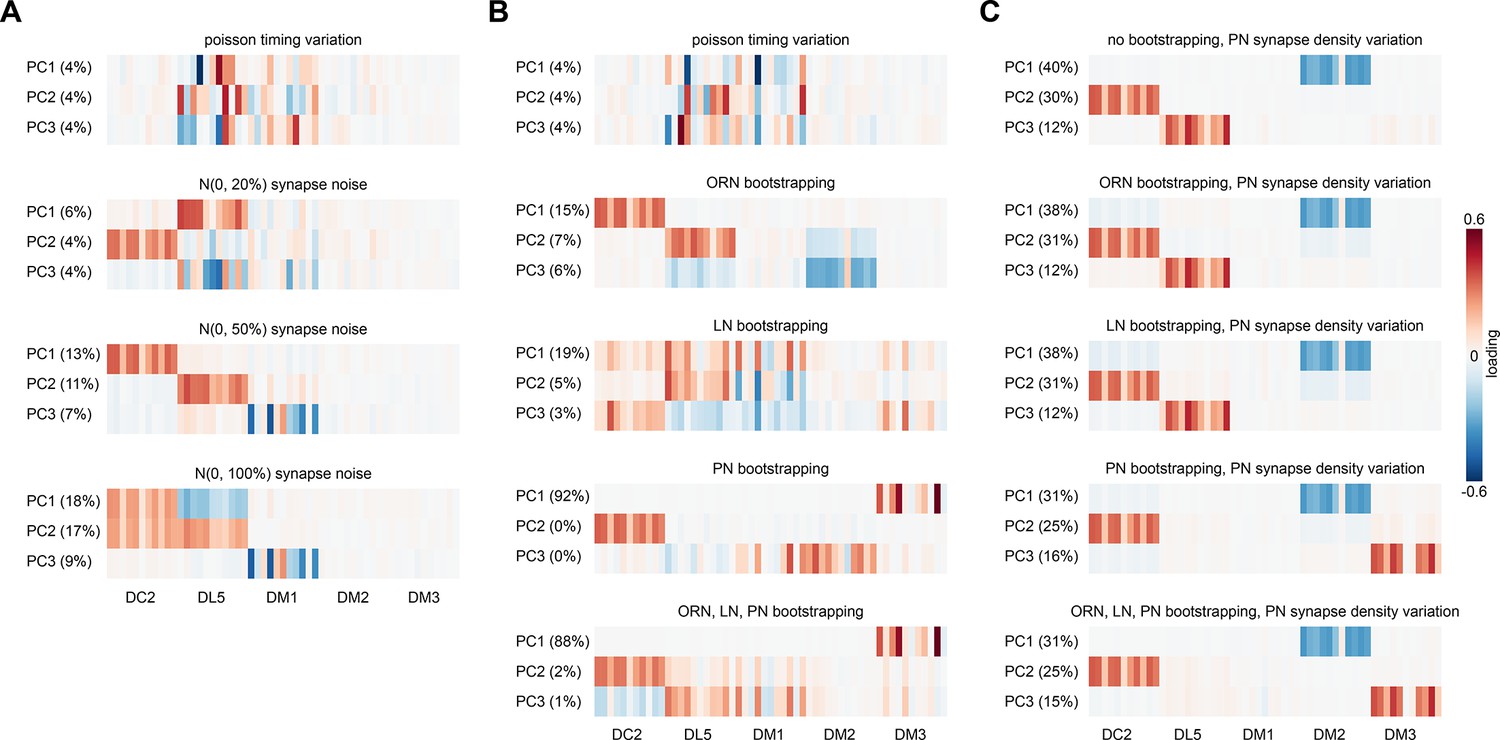
Projection neuron (PN) response PCA loadings under various sources of circuit idiosyncrasy.
(A) Loadings of the principal components of PN glomerulus-odor responses as simulated across antennal lobe (AL) models where Gaussian noise with an SD equal to 0, 20, 50, and 100% of each synapse weight was added to each synaptic weight in the hemibrain data set. (B) Circuit variation coming from bootstrapping of each major AL cell type or all three simultaneously. (C) Circuit variation coming from bootstrap resampling of different cell-type combinations in addition to PN input synapse density resampling as illustrated in Figure 4—figure supplement 4. Each PCA was performed on the outputs of ~1,000 AL simulations.
Figure 4—figure supplement 6
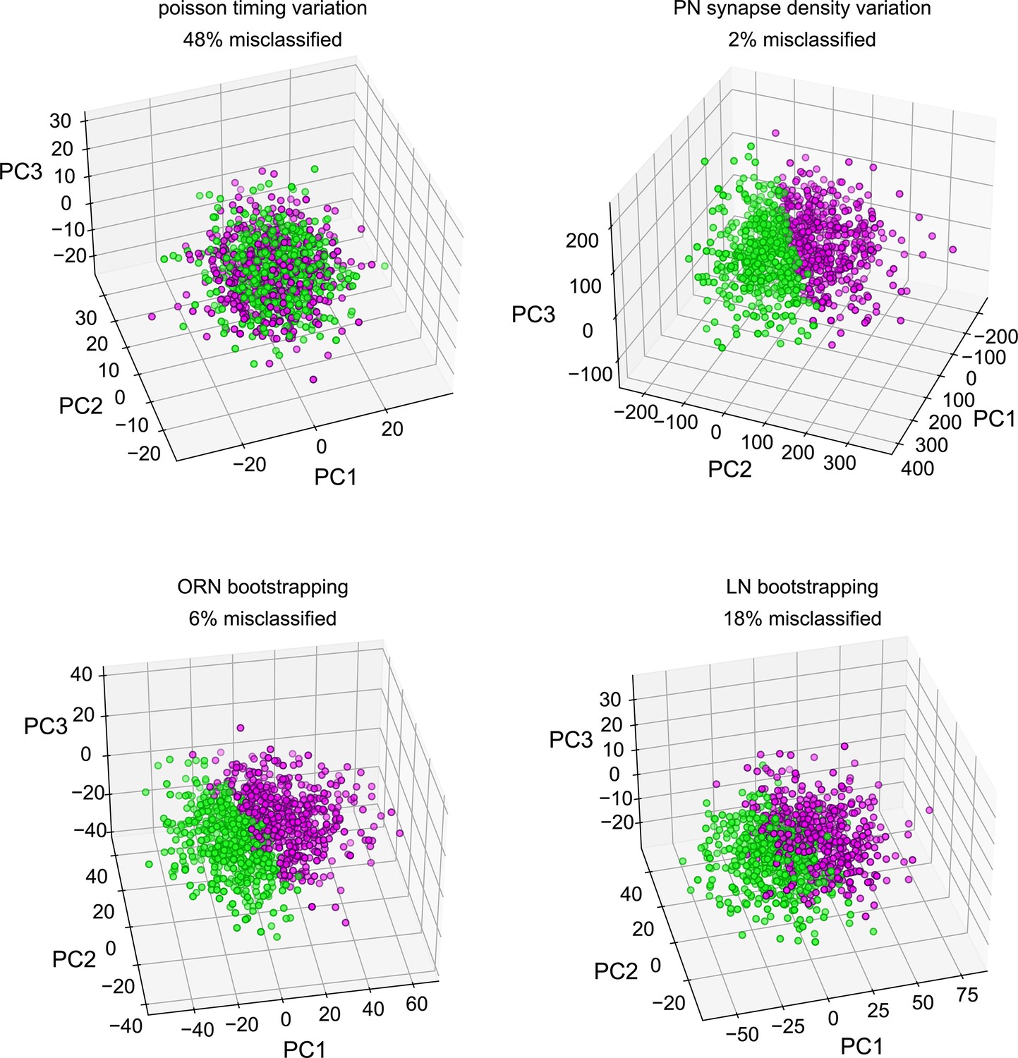
Classifiability of simulated idiosyncratic behavior under different sources of circuit idiosyncrasy.
Simulated projection neuron (PN) odor-glomerulus firing rates projected into their first three principal components. Individual points represent single runs of resampled antennal lobe (AL) models, under four different sources of idiosyncratic variation. PN responses in all odor-glomerulus dimensions were used to calculate simulated behavior scores for each resampled AL by applying the PN calcium-odor-vs.-odor linear model (Figure 2A). Magenta points represent flies with simulated preference for MCH in the top 50%, and green OCT preference. % Misclassification refers to 100% – the accuracy of a linear classifier trained on MCH-vs.-OCT preference in the space of the first three PCs. This measures how much of the variance along the PN calcium-odor-vs.-odor linear model lies outside the first three PCs of simulated PN variation.
Videos
Video 1
Example recording with automated tracking of an odor-vs.-air behavioral assay.
The recent positions of each fly (green line) are shown in different colors. Red bar indicates when the odor stream is turned on.
Video 2
Example recording with automated tracking of an odor-vs.-odor behavioral assay.
The recent positions of each fly (green line) are shown in different colors. Magenta and green bars at right indicate when MCH and OCT are respectively flowing into the top and bottom halves of each arena.
Video 3
Confocal image stack of expanded DC2>Brp-Short.
Magenta is nc82 stain, green is Or13a>Brp-Short. Frames are z-slices spaced at 0.54 µm. Image height corresponds to a post-expansion field of view of 107 × 90 µm (~2.5× linear expansion factor).
Video 4
Simulated antennal lobe (AL) connectivity matrices.
Left: glomerular density resampling. Each frame corresponds to the hemibrain connectome synaptic weights, rescaled according to a sample from the relationship between synapse count and volume parameterized in Figure 4—figure supplement 4. Middle: olfactory receptor neuron (ORN) bootstrapping. Each frame corresponds to the hemibrain connectome synaptic weights, but with the population of ORNs projecting to each glomerulus resampled with replacement. Right: local neuron (LN) bootstrapping. Each frame corresponds to the hemibrain connectome synaptic weights, but with the population of LNs resampled with replacement.
Tables
Table 1
Calcium and Brp-Short – behavior model statistics.
| Behavior neasured | Neural predictor | Figure panel | n | β0 | β1 | R2 | p-Value |
|---|---|---|---|---|---|---|---|
| OCT vs. AIR | PN calcium PC 1 | Figure 2—figure supplement 1A | 18 | –0.26 | –0.079 | 0.16 | 0.099 |
| OCT vs. AIR | PN calcium average all dimensions | Figure 1—figure supplement 10I | 53 | –0.051 | –0.38 | 0.098 | 0.022 |
| OCT vs. AIR | ORN calcium PC 1 | Figure 1—figure supplement 10B | 30 | –0.29 | –0.053 | 0.23 | 0.007 |
| OCT vs. AIR | ORN calcium average all dimensions | Figure 1—figure supplement 10E | 30 | –0.032 | –0.71 | 0.25 | 0.005 |
| OCT vs. MCH | PN calcium PC 2 | Figure 2—figure supplement 1C | 47 | –0.058 | –0.081 | 0.15 | 0.006 |
| OCT vs. MCH | PN calcium DM2–DC2 (% difference) | Figure 2I | 69 | –0.032 | –0.0018 | 0.12 | 0.004 |
| OCT vs. MCH | ORN calcium PC 1 | Figure 1L | 35 | –0.14 | –0.027 | 0.031 | 0.32 |
| OCT vs. MCH | ORN Brp-Short PC 2 (train data only) | Figure 3—figure supplement 1I | 22 | –0.087 | 0.017 | 0.22 | 0.028 |
| OCT vs. MCH | ORN Brp-Short PC 2 (all data) | Figure 3F | 53 | –0.019 | 0.012 | 0.088 | 0.031 |
-
MCH, 4-methylcyclohexanol; OCT, 3-octanol; ORN, olfactory receptor neuron; PC, principal component; PN, projection neuron.
Table 2
Typical electrophysiology features of antennal lobe cell types, used as model parameters.
| Parameter | Olfactory receptor neurons | Local neurons | Projection neurons |
|---|---|---|---|
| Membrane resting potential | –70 mV (Dubin and Harris, 1997) | –50 mV (Seki et al., 2010) | –55 mV (Jeanne and Wilson, 2015) |
| Action potential threshold | –50 mV (Dubin and Harris, 1997) | –40 mV (Seki et al., 2010) | –40 mV (Jeanne and Wilson, 2015) |
| Action potential minimum | –70 mV (Cao et al., 2016) | –60 mV (Seki et al., 2010) | –55 mV (Jeanne and Wilson, 2015) |
| Action potential maximum | 0 mV (Dubin and Harris, 1997) | 0 mV (Seki et al., 2010) | –30 mV (Wilson and Laurent, 2005) |
| Action potential duration | 2 ms (Jeanne and Wilson, 2015) | 4 ms (Seki et al., 2010) | 2 ms (Jeanne and Wilson, 2015) |
| Membrane capacitance | 73 pF (assumed = projection neurons) | 64 pF (Huang et al., 2018) | 73 pF (Huang et al., 2018) |
| Membrane resistance | 1.8 GOhm (Dubin and Harris, 1997) | 1 GOhm (Seki et al., 2010) | 0.3 GOhm (Jeanne and Wilson, 2015) |
Key resources table
| Reagent type (species) or resource | Designation | Source or reference | Identifiers | Additional information |
|---|---|---|---|---|
| Genetic reagent (Drosophila melanogaster) | P{20XUAS-IVS-GCaMP6m}attP40 | Bloomington Drosophila Stock Center | RRID:BDSC_42748 | |
| Genetic reagent (D. melanogaster) | w[*]; P{w[+mC]=Or13a-GAL4.F}40.1 | Bloomington Drosophila Stock Center | RRID:BDSC_9945 | |
| Genetic reagent (D. melanogaster) | w[*]; P{w[+mC]=Or19a-GAL4.F}61.1 | Bloomington Drosophila Stock Center | RRID:BDSC_9947 | |
| Genetic reagent (D. melanogaster) | w[*]; P{w[+mC]=Or22a-GAL4.7.717}14.2 | Bloomington Drosophila Stock Center | RRID:BDSC_9951 | |
| Genetic reagent (D. melanogaster) | w[*]; P{w[+mC]=Orco-GAL4.W}11.17; TM2/TM6B, Tb[1] | Bloomington Drosophila Stock Center | RRID:BDSC_26818 | |
| Genetic reagent (D. melanogaster) | isokh11 isogenic line | https://doi.org/10.1073/pnas.1901623116 | Honegger et al., 2020 | |
| Genetic reagent (D. melanogaster) | GH146-Gal4 | https://doi.org/10.1073/pnas.1901623116 | Gift of Y. Zhong (Honegger et al., 2020) | |
| Genetic reagent (D. melanogaster) | w; UAS-Brp-Short-mStrawberry; UAS-mCD8-GFP; + | https://doi.org/10.7554/eLife.03726 | Gift of T. Mosca (Mosca and Luo, 2014) | |
| Antibody | Anti-nc82 (mouse monoclonal) | Developmental Studies Hybridoma Bank | DSHB:nc82; RRID:AB_2314866 | (1:40) |
| Antibody | Anti-GFP (chicken polyclonal) | Aves Labs | Aves Labs:GFP-1020; RRID:AB_10000240 | (1:1000) |
| Antibody | Anti-mStrawberry (rabbit polyclonal) | biorbyt | Biorbyt:orb256074 | (1:1000) |
| Antibody | Atto 647N-conjugated anti-mouse (goat polyclonal) | MilliporeSigma | Sigma-Aldrich:50185; RRID:AB_1137661 | (1:250) |
| Antibody | Alexa Fluor 568-conjugated anti-rabbit (goat polyclonal) | Thermo Fisher | Thermo Fisher Scientific:A-11011; RRID:AB_143157 | (1:250) |
| Antibody | Alexa Fluor 488-conjugated anti-chicken (goat polyclonal) | Thermo Fisher | Thermo Fisher Scientific:A-11039; RRID:AB_2534096 | (1:250) |
| Chemical compound, drug | 2-Heptanone | MilliporeSigma | CAS #110-43-0 | |
| Chemical compound, drug | 1-Pentanol | MilliporeSigma | CAS #71-41-0 | |
| Chemical compound, drug | 3-Octanol | MilliporeSigma | CAS #589-98-0 | |
| Chemical compound, drug | Hexyl-acetate | MilliporeSigma | CAS #142-92-7 | |
| Chemical compound, drug | 4-Methylcyclohexanol | MilliporeSigma | CAS #589-91-3 | |
| Chemical compound, drug | Pentyl acetate | MilliporeSigma | CAS #628-63-7 | |
| Chemical compound, drug | 1-Butanol | MilliporeSigma | CAS #71-36-3 | |
| Chemical compound, drug | Ethyl lactate | MilliporeSigma | CAS #97-64-3 | |
| Chemical compound, drug | Geranyl acetate | Millipore Sigma | CAS #105-87-3 | |
| Chemical compound, drug | 1-Hexanol | MilliporeSigma | CAS #111-27-34 | |
| Chemical compound, drug | Citronella java essential oil | Aura Cacia | Aura Cacia:191112 | |
| Software, algorithm | Python (version 3.6) | Python Software Foundation | RRID:SCR_008394 | |
| Software, algorithm | MathWorks, MATLAB pca documentation, 2018 | RRID:SCR_001622 |
Additional files
Download links
A two-part list of links to download the article, or parts of the article, in various formats.
Downloads (link to download the article as PDF)
Open citations (links to open the citations from this article in various online reference manager services)
Cite this article (links to download the citations from this article in formats compatible with various reference manager tools)
A neural correlate of individual odor preference in Drosophila
eLife 12:RP90511.
https://doi.org/10.7554/eLife.90511.4


