Research Article

Neuroscience

Statistical learning shapes pain perception and prediction independently of external cues

Computational and Biological Learning Unit, Department of Engineering, University of Cambridge, United Kingdom
Applied Computational Psychiatry Lab, Max Planck Centre for Computational Psychiatry and Ageing Research, Queen Square Institute of Neurology and Mental Health Neuroscience Department, Division of Psychiatry, University College London, United Kingdom
MRC Cognition and Brain Sciences Unit, University of Cambridge, United Kingdom
Wellcome Centre for Integrative Neuroimaging, John Radcliﬀe Hospital, Headington, United Kingdom
Center for Information and Neural Networks (CiNet), Japan

Jul 10, 2024

https://doi.org/10.7554/eLife.90634.3

Open access
Copyright information

Figures
Tables
Additional files

20 figures, 10 tables and 1 additional file

Figures

Figure 1

Download asset Open asset

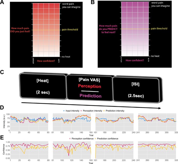
Task design.

On each trial, each participant received a thermal stimulus lasting 2s from a sequence of intensities. This was followed by a perception (A) or a prediction (B) input screen, where the y-axis indicates the level of perceived/predicted intensity (0–100) centred around participant’s pain threshold, and the x-axis indicates the level of confidence in one’s perception (0–1). The inter-stimulus interval (ISI; black screen) lasted 2.5s (trial example in C). (D) Example intensity sequences are plotted in green, participant’s perception and prediction responses are in red and black, respectively. (E) Participant’s confidence rating for perception (red) and prediction (black) trials.

Figure 2

Download asset Open asset

Participant’s model-naive performance in the task.

Violin plots of participant root mean square error (RMSE) for each condition for A: rating and B: prediction responses as compared with the input. Lower and upper hinges correspond to the first and third quartiles of partipants’ errors (the upper/lower whisker extends from the hinge to the largest/smallest value no further than 1.5 * ”Interquartile range” from the hinge); the line in the box corresponds to the median. Each condition has N=27 particpants.

Figure 3

Download asset Open asset

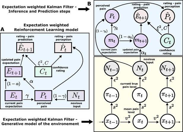
Expectation weighted models.

Computational models used in the main analysis to capture participants’ pain perception ( ${\hat{P}}_{t}$ ) and prediction ( ${\hat{E}}_{t + 1}$ ) ratings. Both types of ratings are affected by confidence rating ( $C_{t})$ ) on each trial. (A) In the reinforcement learning model, participant’s pain perception ( $P_{t}$ ) is taken to be weighted sum of the current noxious input ( $N_{t}$ ) and their current pain expectation ( $E_{t}$ ). Following the noxious input, participant updates their pain expectation ( $E_{t + 1}$ ). (B) In the Kalman filter model, a generative model of the environment is assumed (yellow background) - where the mean pain level ( $x_{t}$ ) evolves according to a Gaussian random walk (volatility $v^{2}$ ). The true pain level on each trial ( $π_{t}$ ) is then drawn from a Gaussian (stochasticity $s^{2}$ ). Lastly, the noxious input, $N_{t}$ , is assumed an imperfect indicator of the true pain level (subjective noise $ϵ^{2}$ ). Inference and prediction steps are depicted in a blue box. Participant’s perceived pain is a weighted sum of expectation about the pain level ( $m_{t}$ ) and current noxious input ( $N_{t}$ ). Following each observation, $N_{t}$ , participant updates their expectation about the pain level ( $m_{t + 1}$ ).

Figure 4

Download asset Open asset

Confidence scaling factor demonstration.

(**A–F**) For a range of values of the confidence scaling factor $C$ , we simulated a set of typical responses a participant would make for various levels of confidence ratings. The belief about the mean of the sequence is set at 50, while the response noise at 10. The confidence scaling factor $C$ effectively scales the response noise, adding or reducing response uncertainty. (**G–L**) The effect of different levels of parameter $C$ on noise scaling. As $C$ increases the effect of confidence is diminished.

Figure 5

Download asset Open asset

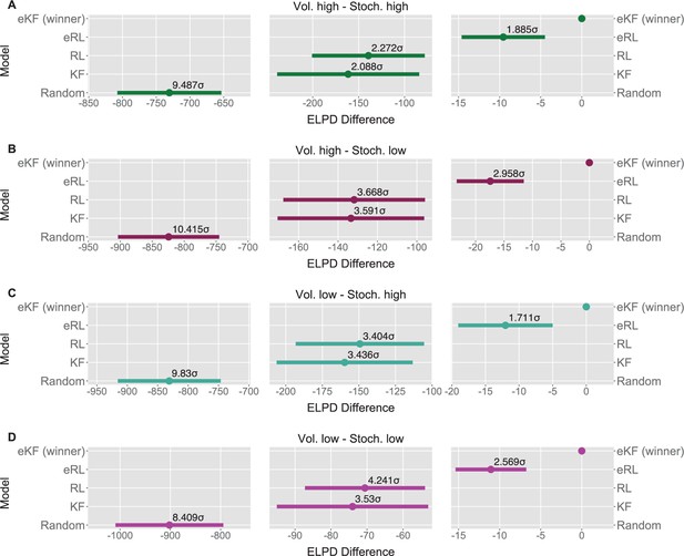
Model comparison for each sequence condition (**A–D**).

The dots indicate the expected log point-wise predictive density (ELPD) difference between the winning model (eKF - expectation weighted Kalman filter) and every other model. The line indicates the standard error (SE) of the difference. The non-winning models’ ELPD differences are annotated with the ratio between the ELPD difference and SE indicating the sigma effect, a significance heuristic.

Figure 6

Download asset Open asset

The effect of the confidence scaling factor on noise scaling for each condition.

(**A–D**) Each coloured line corresponds to one participant, with the black line indicating the mean across all participants. The mean slope for each condition is annotated.

Appendix 1—figure 1

Download asset Open asset

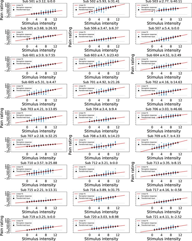
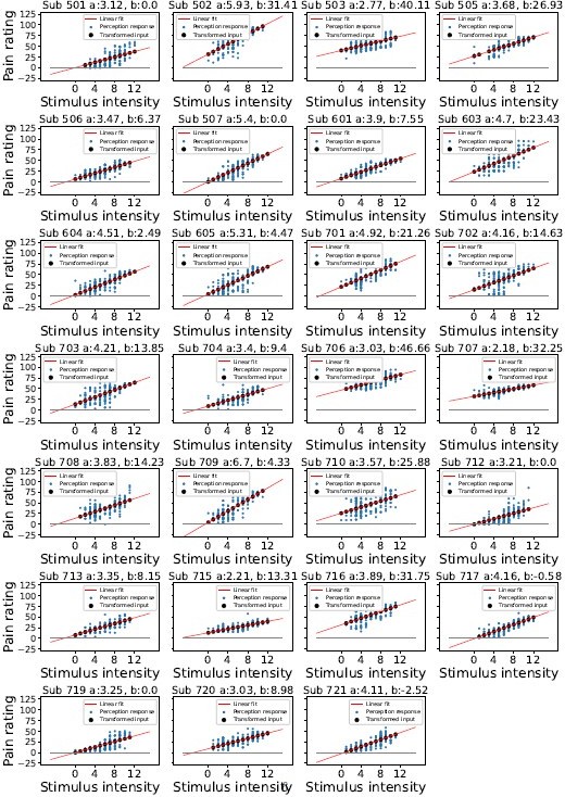
Linear transformation of the input at perception trials.

Blue dots indicate participant’s perception responses for a given level of stimulus intensity, black dots indicate transformed intensity values, a linear least squares regression was performed to achieve the best fitting line through participant’s responses as shown in red, the intercept was constrained>0.

Appendix 1—figure 2

Download asset Open asset

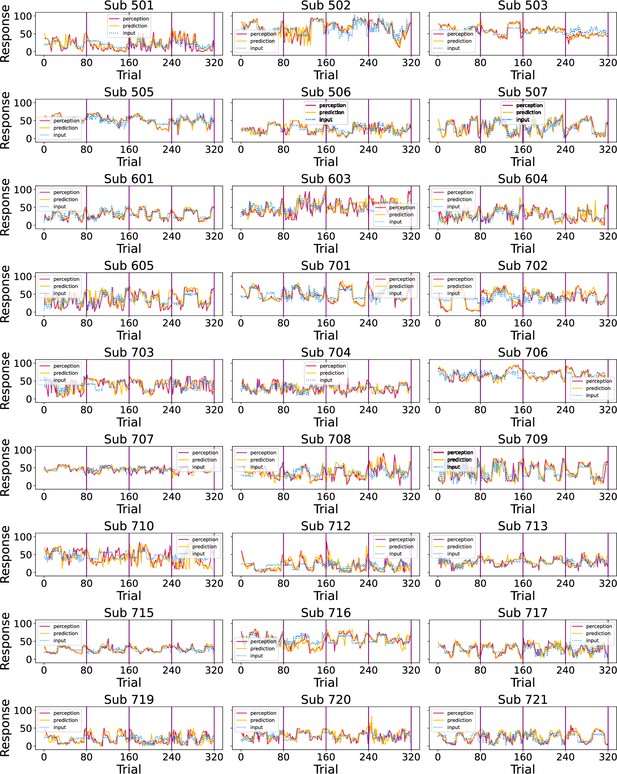
Participants’ responses (red - perception; green - prediction) to the noxious input (dotted line) sequences.

Vertical purple lines mark the end of each condition.

Appendix 1—figure 3

Download asset Open asset

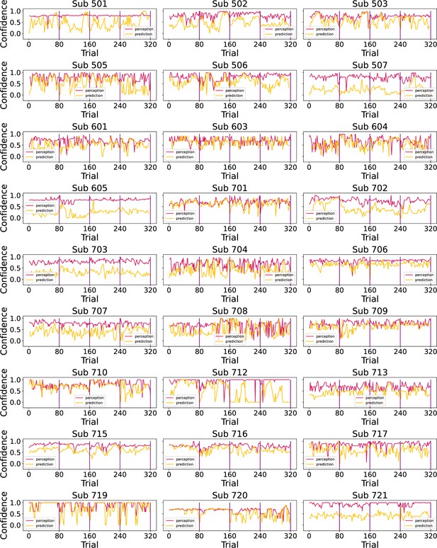
Participants’ confidence ratings (red - perception; green - prediction) during the task.

Vertical purple lines mark the end of each condition.

Appendix 1—figure 4

Download asset Open asset

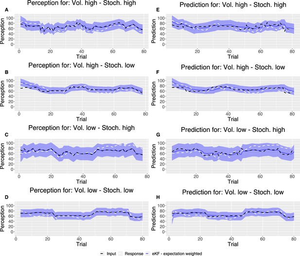
Example plot of the input sequences (black) for each condition, one participant’s responses (white) and the winning, expectation weighted Kalman filter (eKF), model predictions (blue) including 95% confidence intervals (shaded blue) for (**A–D**) perception and (**E–H**) prediction.

Appendix 1—figure 5

Download asset Open asset

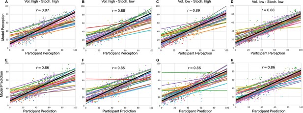
Model responses against participants’ responses for each condition and each response type (**A–D**) perception and (**E–H**) prediction.

The annotated value is the grand mean correlation across subjects for each condition and response type.

Appendix 1—figure 6

Download asset Open asset

Parameter recovery average SD for: (A) eRL; (B) RL; (C) eKF; (D) KF; (E) Random model.

The average SD is plotted as a function of simulation number averaged across 500 permutations of ≈100 simulations. The coloured shading corresponds to 1 SD around the average error.

Appendix 1—figure 7

Download asset Open asset

Parameter recovery scatter plot for expectation weighted reinforcement learning (eRL) model from ≈100 simulations for: (A) ɑ; (B) ɣ; (C) ξ; (D) E0; (E) C parameter.

Appendix 1—figure 8

Download asset Open asset

Parameter recovery scatter plot for reinforcement learning (RL) model from ≈100 simulations for: (A) ɑ; (B) ξ; (C) E0; (D) C parameter.

Appendix 1—figure 9

Download asset Open asset

Parameter recovery scatter plot for expectation weighted Kalman filter (eKF) model from ≈100 simulations for: (A) ε; (B) s; (C) v; (D) ξ; (E) E0; (F) w0; (G) C parameter.

Appendix 1—figure 10

Download asset Open asset

Parameter recovery scatter plot for Kalman filter (KF) model from ≈100 simulations for: (A) s; (B) v; (C) ξ; (D) E0; (E) w0; (F) C parameter.

Appendix 1—figure 11

Download asset Open asset

Parameter recovery scatter plot for random model from ≈100 simulations for: (A) ξ; (B) R; (C) C parameter.

Appendix 1—figure 12

Download asset Open asset

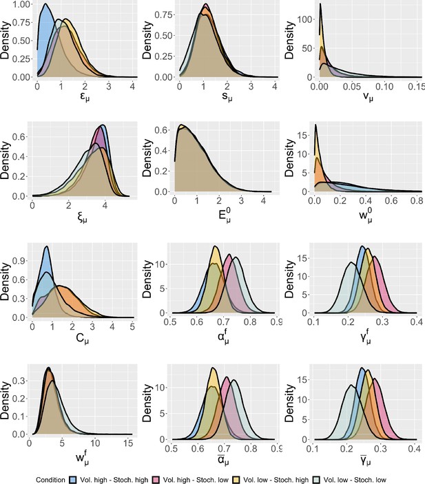
Group-level distributions for parameters for each condition for the expectation weighted Kalman filter (eKF) model.

Appendix 1—figure 13

Download asset Open asset

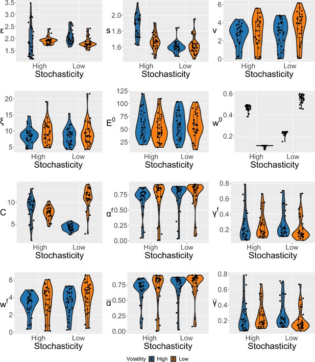
Violin plots (and box-plots) of individual-level parameters for each condition in the winning expectation weighted Kalman filter (eKF) model.

Lower and upper hinges correspond to the first and third quartiles of partipants’ errors (the upper/lower whisker extends from the hinge to the largest/smallest value no further than 1.5 * ”Interquartile range” from the hinge); the line in the box corresponds to the median. Each condition has N=27 particpants.

Author response image 1

Download asset Open asset

Tables

Appendix 1—table 1

Within-subjects effects from repeated measures ANOVA of participant’s RMSE scores with stochasticity, volatility, and response type factors.

SS - sum of squares, MS - mean square, RMSE - root mean square error

Effect	SS	df	MS	F	p	$η^{2}$	$η_{p}^{2}$
Volatility	10.714	1	10.714	0.960	0.336	0.007	0.036
Residuals	290.166	26	11.160
Stochasticity	113.964	1	113.964	19.939	<0.001*	0.074	0.434
Residuals	148.603	26	5.715
Type	365.000	1	365.000	85.109	<0.001*	0.237	0.766
Residuals	111.503	26	4.289
Volatility × stochasticity	0.006	1	0.006	5.688e^-4	0.981	3.723e^-6	2.188e^-5
Residuals	261.912	26	10.074
Volatility × type	7.313	1	7.313	3.196	0.085	0.005	0.109
Residuals	59.487	26	2.288
Stochasticity × type	63.662	1	63.662	29.842	<0.001*	0.041	0.534
Residuals	55.466	26	2.133
Volatility × stochasticity × type	1.356	1	1.356	0.704	0.409	8.807e^-4	0.026
Residuals	50.060	26	1.925

* indicates statistical significance at 0.05 level.

Appendix 1—table 2

Post hoc comparisons for the repeated measures ANOVA’s interaction effect of stochasticity × type.

			95%CI for mean diff.
		Mean diff.	Lower	Upper	SE	t	p_bonf
High, perception	Low, perception	0.367	−0.687	1.421	0.381	0.963	1.000
	High, prediction	−3.686	−4.636	−2.735	0.345	−10.688	<0.001*
	Low, prediction	−1.147	−2.329	0.034	0.430	−2.665	0.062
Low, perception	High, prediction	−4.053	−5.234	−2.871	0.430	−9.415	<0.001*
	Low, prediction	−1.514	−2.464	−0.564	0.345	−4.390	<0.001*
High, prediction	Low, prediction	2.539	1.484	3.593	0.381	6.658	<0.001*

* indicates statistical significance at 0.05 level.

Appendix 1—table 3

Pearson correlation coeﬃcient $r$ (SD) from the parameter recovery analysis for each model.

	eRL
	$α$	$γ$	$ξ$	$E^{0}$	$C$
$r$ (SD)	0.685 (0.113)	0.92 (0.049)	0.993 (0.005)	0.723 (0.093)	0.481 (0.131)
	RL
	$α$	$ξ$	$E^{0}$	$C$
$r$ (SD)	0.842 (0.081)	0.993 (0.004)	0.625 (0.107)	0.455 (0.133)
	eKF
	$ϵ$	$s$	$v$	$ξ$	$E^{0}$	$w^{0}$	$C$
$r$ (SD)	0.742 (0.1)	0.531 (0.13)	0.745 (0.09)	0.986 (0.075)	0.849 (0.118)	0.309 (0.179)	0.472 (0.123)
	KF
	$s$	$v$	$ξ$	$E^{0}$	$w^{0}$	$C$
$r$ (SD)	0.605 (0.129)	0.589 (0.117)	0.993 (0.005)	0.585 (0.157)	0.298 (0.18)	0.442 (0.146)
	Random model
	$ξ$	$R$	$C$
$r$ (SD)	0.996 (0.004)	0.999 (0.001)	0.079 (0.206)

Appendix 1—table 4

Confusion matrix from the model recovery analysis based on ≈100 simulations.

The y-axis indicates which model simulated the dataset, while the x-axis indicates which model ﬁt the data based on leave-one-out information criterion (LOOIC).

		eRL	RL	eKF	KF	Random
Simulated	eRL	0.327	0.173	0.404	0.096	0.000
	RL	0.223	0.234	0.223	0.319	0.000
	eKF	0.382	0.067	0.427	0.124	0.000
	KF	0.229	0.281	0.281	0.208	0.000
	Random	0.292	0.000	0.358	0.000	0.349
	Fit

Appendix 1—table 5

Model comparison results for each condition.

Condition	Model name	ELPD diﬀerence	SE diﬀerence	Sigma eﬀect	LOOIC
Vol. high Stoch. high	eKF - expectation weighted	0.000	0.000		15748.389
	eRL - expectation weighted	–9.560	5.071	1.885	15767.509
	RL	–139.407	61.362	2.272	16027.202
	KF	–161.444	77.335	2.088	16071.277
	Random response	–730.600	77.009	9.487	17209.588
Vol. high Stoch. low	eKF - expectation weighted	0.000	0.000		15682.115
	eRL - expectation weighted	–17.439	5.896	2.958	15716.993
	RL	–131.817	35.936	3.668	15945.749
	KF	–133.464	37.171	3.591	15949.042
	Random response	–824.346	79.148	10.415	17330.807
Vol. low Stoch. high	eKF - expectation weighted	0.000	0.000		15990.114
	eRL - expectation weighted	–12.027	7.029	1.711	16014.169
	RL	–149.338	43.874	3.404	16288.789
	KF	–159.738	46.485	3.436	16309.590
	Random response	–831.096	84.549	9.830	17652.306
Vol. low Stoch. low	eKF - expectation weighted	0.000	0.000		15904.936
	eRL - expectation weighted	–11.068	4.309	2.569	15927.072
	RL	–70.588	16.643	4.241	16046.111
	KF	–74.031	20.972	3.530	16052.997
	Random response	–901.792	107.244	8.409	17708.519

Appendix 1—table 6

Bulk and tail effective sample size (ESS) values for vol. high - stoch. high.

Model	Param.	ESS (bulk)	ESS (tail)
eRL	$α$	58.166	47.491
	$C$	90.5	79.142
	$E^{0}$	54.655	137.729
	$ξ$	31.233	47.726
	$γ$	39.509	49.335
RL	$α$	56.22	36.057
	$C$	99.642	52.599
	$E^{0}$	126.757	467.373
	$ξ$	31.322	36.92
eKF	$C$	89.281	83.274
	$E^{0}$	37.723	103.977
	$ϵ$	94.203	429.332
	$v$	53.099	41.511
	$s$	1665.566	4593.161
	$w^{0}$	616458.467	467603.626
	$ξ$	31.322	47.1
KF	$C$	101.584	55.345
	$E^{0}$	122.76	512.134
	$v$	114.644	54.015
	$s$	438.028	730.579
	$w^{0}$	904.643	6759.804
	$ξ$	31.457	36.763
Random	$R$	27.939	33.982
	$C$	397.862	259.967
	$ξ$	32.334	41.271

Appendix 1—table 7

Bulk and tail effective sample size (ESS) values for vol. high - stoch. low.

Model	Param.	ESS (bulk)	ESS (tail)
eRL	$α$	86.32	60.849
	$C$	235.396	373.736
	$E^{0}$	43.489	109.903
	$ξ$	30.471	36.664
	$γ$	42.125	55.178
RL	$α$	49.221	40.877
	$C$	328.761	455.542
	$E^{0}$	63.341	111.689
	$ξ$	30.304	38.063
eKF	$C$	227.813	363.944
	$E^{0}$	33.393	104.395
	$ϵ$	376.691	1218.299
	$v$	45.861	37.486
	$s$	99526.69	148393.383
	$w^{0}$	567627.288	634817.458
	$ξ$	30.438	36.66
KF	$C$	328.005	448.632
	$E^{0}$	57.467	124.471
	$v$	293.426	480.255
	$s$	164.454	598.211
	$w^{0}$	412979.973	354163.251
	$ξ$	30.16	38.105
Random	$R$	28.397	32.922
	$C$	1794.614	1170.459
	$ξ$	30.204	34.896

Appendix 1—table 8

Bulk and tail effective sample size (ESS) values for vol. low - stoch. high.

Model	Param.	ESS (bulk)	ESS (tail)
eRL	$α$	43.312	40.66
	$C$	248.885	434.44
	$E^{0}$	49.006	85.409
	$ξ$	29.68	34.909
	$γ$	45.37	52.755
RL	$α$	39.911	35.351
	$C$	433.949	435.575
	$E^{0}$	181.442	618.317
	$ξ$	29.527	36.192
eKF	$C$	248.848	418.003
	$E^{0}$	35.363	51.728
	$ϵ$	1272.838	2427.211
	$v$	41.144	40.915
	$s$	2399.657	6854.212
	$w^{0}$	612283.163	531588.25
	$ξ$	29.699	34.762
KF	$C$	423.339	417.747
	$E^{0}$	88.749	302.863
	$v$	58.795	47.015
	$s$	206.969	672.666
	$w^{0}$	499152.469	573964.793
	$ξ$	29.511	36.341
Random	$R$	27.892	32.919
	$C$	269.239	106.139
	$ξ$	29.69	44.38

Appendix 1—table 9

Bulk and tail effective sample size (ESS) values for vol. low - stoch. low.

Model	Param.	ESS (bulk)	ESS (tail)
eRL	$α$	57.116	40.932
	$C$	162.472	129.413
	$E^{0}$	43.707	117.295
	$ξ$	29.632	34.486
	$γ$	65.497	151.548
RL	$α$	45.892	37.244
	$C$	158.681	98.898
	$E^{0}$	80.406	441.719
	$ξ$	29.558	35.077
eKF	$C$	149.16	126.209
	$E^{0}$	38.88	73.732
	$ϵ$	653.635	1473.554
	$v$	48.883	43.445
	$s$	2263.547	9318.066
	$w^{0}$	635517.969	313426.188
	$ξ$	29.699	34.721
KF	$C$	158.729	105.929
	$E^{0}$	71.438	457.431
	$v$	91.988	69.957
	$s$	287.835	895.249
	$w^{0}$	527620.655	587092.529
	$ξ$	29.527	35.147
Random	$R$	28.474	38.123
	$C$	2426.581	1279.66
	$ξ$	29.532	34.731

Appendix 1—table 10

Model diagnostics for each condition - estimated Bayesian fraction of missing information (E-BFMI), number of divergent transition E-BFMI values per chain.

Condition	Model	E-BFMI values
HVHS	eRL	0.696 0.713 0.695 0.691
	RL	0.76 0.748 0.771 0.806
	eKF	0.755 0.767 0.771 0.759
	KF	0.633 0.596 0.547 0.563
	Random	0.842 0.851 0.843 0.835
HVLS	eRL	0.689 0.76 0.69 0.689
	RL	0.624 0.688 0.688 0.685
	eKF	0.741 0.764 0.753 0.779
	KF	0.654 0.734 0.689 0.674
	Random	0.883 0.779 0.836 0.833
LVHS	eRL	0.73 0.732 0.728 0.702
	RL	0.719 0.714 0.742 0.7
	eKF	0.753 0.755 0.792 0.766
	KF	0.75 0.768 0.729 0.754
	Random	0.864 0.849 0.883 0.845
LVLS	eRL	0.764 0.762 0.75 0.764
	RL	0.714 0.764 0.719 0.697
	eKF	0.783 0.751 0.772 0.77
	KF	0.705 0.695 0.702 0.726
	Random	0.835 0.829 0.852 0.847

Additional files

MDAR checklist: https://cdn.elifesciences.org/articles/90634/elife-90634-mdarchecklist1-v1.docx
Download elife-90634-mdarchecklist1-v1.docx

Download links

A two-part list of links to download the article, or parts of the article, in various formats.

Downloads (link to download the article as PDF)

Article PDF

Open citations (links to open the citations from this article in various online reference manager services)

Mendeley

Cite this article (links to download the citations from this article in formats compatible with various reference manager tools)

Jakub Onysk
Nicholas Gregory
Mia Whitefield
Maeghal Jain
Georgia Turner
Ben Seymour
Flavia Mancini

(2024)

Statistical learning shapes pain perception and prediction independently of external cues

eLife 12:RP90634.

https://doi.org/10.7554/eLife.90634.3

Figures

Task design.

Participant’s model-naive performance in the task.

Expectation weighted models.

Confidence scaling factor demonstration.

Model comparison for each sequence condition (A–D).

The effect of the confidence scaling factor on noise scaling for each condition.

Linear transformation of the input at perception trials.

Participants’ responses (red - perception; green - prediction) to the noxious input (dotted line) sequences.

Participants’ confidence ratings (red - perception; green - prediction) during the task.

Example plot of the input sequences (black) for each condition, one participant’s responses (white) and the winning, expectation weighted Kalman filter (eKF), model predictions (blue) including 95% confidence intervals (shaded blue) for (A–D) perception and (E–H) prediction.

Model responses against participants’ responses for each condition and each response type (A–D) perception and (E–H) prediction.

Parameter recovery average SD for: (A) eRL; (B) RL; (C) eKF; (D) KF; (E) Random model.

Parameter recovery scatter plot for expectation weighted reinforcement learning (eRL) model from ≈100 simulations for: (A) ɑ; (B) ɣ; (C) ξ; (D) E0; (E) C parameter.

Parameter recovery scatter plot for reinforcement learning (RL) model from ≈100 simulations for: (A) ɑ; (B) ξ; (C) E0; (D) C parameter.

Parameter recovery scatter plot for expectation weighted Kalman filter (eKF) model from ≈100 simulations for: (A) ε; (B) s; (C) v; (D) ξ; (E) E0; (F) w0; (G) C parameter.

Parameter recovery scatter plot for Kalman filter (KF) model from ≈100 simulations for: (A) s; (B) v; (C) ξ; (D) E0; (E) w0; (F) C parameter.

Parameter recovery scatter plot for random model from ≈100 simulations for: (A) ξ; (B) R; (C) C parameter.

Group-level distributions for parameters for each condition for the expectation weighted Kalman filter (eKF) model.

Violin plots (and box-plots) of individual-level parameters for each condition in the winning expectation weighted Kalman filter (eKF) model.

Stimulis intensity transformation.

Tables

Within-subjects effects from repeated measures ANOVA of participant’s RMSE scores with stochasticity, volatility, and response type factors.

Post hoc comparisons for the repeated measures ANOVA’s interaction effect of stochasticity × type.

Pearson correlation coeﬃcient $r$ (SD) from the parameter recovery analysis for each model.

Confusion matrix from the model recovery analysis based on ≈100 simulations.

Model comparison results for each condition.

Bulk and tail effective sample size (ESS) values for vol. high - stoch. high.

Bulk and tail effective sample size (ESS) values for vol. high - stoch. low.

Bulk and tail effective sample size (ESS) values for vol. low - stoch. high.

Bulk and tail effective sample size (ESS) values for vol. low - stoch. low.

Model diagnostics for each condition - estimated Bayesian fraction of missing information (E-BFMI), number of divergent transition E-BFMI values per chain.

Additional files

MDAR checklist

Download links

Downloads (link to download the article as PDF)

Open citations (links to open the citations from this article in various online reference manager services)

Cite this article (links to download the citations from this article in formats compatible with various reference manager tools)

Be the first to read new articles from eLife

Share this article

Cite this article

Task design.

Participant’s model-naive performance in the task.

Expectation weighted models.

Confidence scaling factor demonstration.

Model comparison for each sequence condition (A–D).

The effect of the confidence scaling factor on noise scaling for each condition.

Linear transformation of the input at perception trials.

Participants’ responses (red - perception; green - prediction) to the noxious input (dotted line) sequences.

Participants’ confidence ratings (red - perception; green - prediction) during the task.

Example plot of the input sequences (black) for each condition, one participant’s responses (white) and the winning, expectation weighted Kalman filter (eKF), model predictions (blue) including 95% confidence intervals (shaded blue) for (A–D) perception and (E–H) prediction.

Model responses against participants’ responses for each condition and each response type (A–D) perception and (E–H) prediction.

Parameter recovery average SD for: (A) eRL; (B) RL; (C) eKF; (D) KF; (E) Random model.

Parameter recovery scatter plot for expectation weighted reinforcement learning (eRL) model from ≈100 simulations for: (A) ɑ; (B) ɣ; (C) ξ; (D) E0; (E) C parameter.

Parameter recovery scatter plot for reinforcement learning (RL) model from ≈100 simulations for: (A) ɑ; (B) ξ; (C) E0; (D) C parameter.

Parameter recovery scatter plot for expectation weighted Kalman filter (eKF) model from ≈100 simulations for: (A) ε; (B) s; (C) v; (D) ξ; (E) E0; (F) w0; (G) C parameter.

Parameter recovery scatter plot for Kalman filter (KF) model from ≈100 simulations for: (A) s; (B) v; (C) ξ; (D) E0; (E) w0; (F) C parameter.

Parameter recovery scatter plot for random model from ≈100 simulations for: (A) ξ; (B) R; (C) C parameter.

Group-level distributions for parameters for each condition for the expectation weighted Kalman filter (eKF) model.

Violin plots (and box-plots) of individual-level parameters for each condition in the winning expectation weighted Kalman filter (eKF) model.

Stimulis intensity transformation.

Within-subjects effects from repeated measures ANOVA of participant’s RMSE scores with stochasticity, volatility, and response type factors.

Post hoc comparisons for the repeated measures ANOVA’s interaction effect of stochasticity × type.

Pearson correlation coeﬃcient r (SD) from the parameter recovery analysis for each model.

Confusion matrix from the model recovery analysis based on ≈100 simulations.

Model comparison results for each condition.

Bulk and tail effective sample size (ESS) values for vol. high - stoch. high.

Bulk and tail effective sample size (ESS) values for vol. high - stoch. low.

Bulk and tail effective sample size (ESS) values for vol. low - stoch. high.

Bulk and tail effective sample size (ESS) values for vol. low - stoch. low.

Model diagnostics for each condition - estimated Bayesian fraction of missing information (E-BFMI), number of divergent transition E-BFMI values per chain.

MDAR checklist

Downloads (link to download the article as PDF)

Open citations (links to open the citations from this article in various online reference manager services)

Cite this article (links to download the citations from this article in formats compatible with various reference manager tools)

Pearson correlation coeﬃcient $r$ (SD) from the parameter recovery analysis for each model.