Direct observation of the neural computations underlying a single decision
- Zuckerman Mind Brain and Behavior Institute, Columbia University, United States
- Howard Hughes Medical Institute, United States
- Department of Neuroscience, Columbia University, United States
- Kavli Institute, Columbia University, United States
Figures
Figure 1 with 1 supplement

Perceptual decisions are explained by the accumulation of noisy evidence to a stopping bound.
(a) Random dot motion discrimination task. The monkey fixates a central point. After a delay, two peripheral targets appear, followed by the random dot motion. When ready, the monkey reports the net direction of motion by making an eye movement to the corresponding target. Yellow shading indicates the response fields of a subset of neurons in lateral intraparietal cortex (LIP) that we refer to as neurons (target in response field). (b) Mean reaction times (top) and proportion of leftward choices (bottom) plotted as a function of motion strength and direction, indicated by the sign of the coherence: positive is leftward. Data (circles) are from all sessions from monkey M (black, 9684 trials) and monkey J (brown, 8142 trials). Solid lines are fits of a bounded drift-diffusion model. (c) Drift-diffusion model. The decision process is depicted as a race between two accumulators: one integrating momentary evidence for left; the other for right. The momentary samples of evidence are sequential samples from a pair negatively correlated Normal distributions with opposite means (). The decision is terminated when one accumulator reaches its positive bound. The example depicts leftward motion leading to a leftward decision.
Figure 1—figure supplement 1

Effect of motion pulses on behavior (adapted from Figure S1 of Stine et al., 2023).
(a) Choice (bottom) and mean reaction time (top) as a function of motion strength (combined data from the two monkeys; otherwise same conventions as Figure 1b). The two traces show trials in which a leftward (gray) and rightward (black) motion pulse occurred during motion viewing. The pulses (100 ms) had a biasing effect on reaction time (RT) and choice equivalent to shifting the functions left or right by ±1.4% coh (p<0.001, likelihood ratio test). (b) Effect of motion pulses on choices as a function of time from the response. Pulses had a persistent effect on choices, consistent with temporal integration of motion evidence. Shading is ±1 s.e.
Figure 2 with 3 supplements
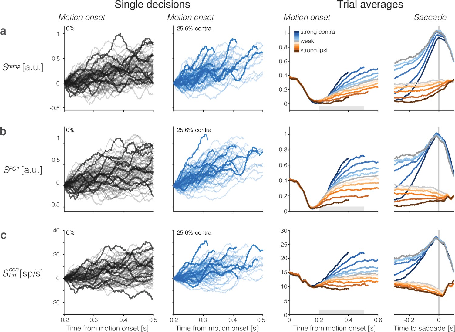
Population responses from lateral intraparietal cortex (LIP) approximate drift-diffusion.
Rows show three types of population signals. The left columns show representative single-trial firing rates during the first 300 ms of evidence accumulation using two motion strengths: 0 and 25.6% coherence toward the left (contralateral) choice target. For visualization, single-trial traces were baseline corrected by subtracting the activity in a 50 ms window around 200 ms. We highlight several trials with thick traces (same trials in a–c). The right columns show the across-trial average responses for each coherence and direction. Motion strength and direction are indicated by color (legend) and aligned to motion onset (left) or saccade initiation (right). The gray bars under the motion-aligned averages indicate the 300 ms epoch used in the display of the single-trial responses (left panels). The epoch begins when LIP first registers a signal related to the strength and direction of motion. Except for saccade-aligned response, trials are cut off 100 ms before saccade initiation. Error trials are excluded from the saccade-aligned averages, only. (a) Ramp coding direction. The weight vector is established by regression to ramps from -1 to +1 over the period of putative integration, from 200 ms after motion onset to 100 ms before saccade initiation (see Figure 2—figure supplement 1). Only trials ending in left (contralateral) choices are used in the regression. (b) First principal component (PC1) coding direction. (c) Average firing rates of the subset of neurons that represent the left (contralateral) target. The weight vector consists of for each of the neurons and 0 for all other neurons. Note the similarity of both the single-trial traces and the response averages produced by the different weighting strategies.
Figure 2—figure supplement 1
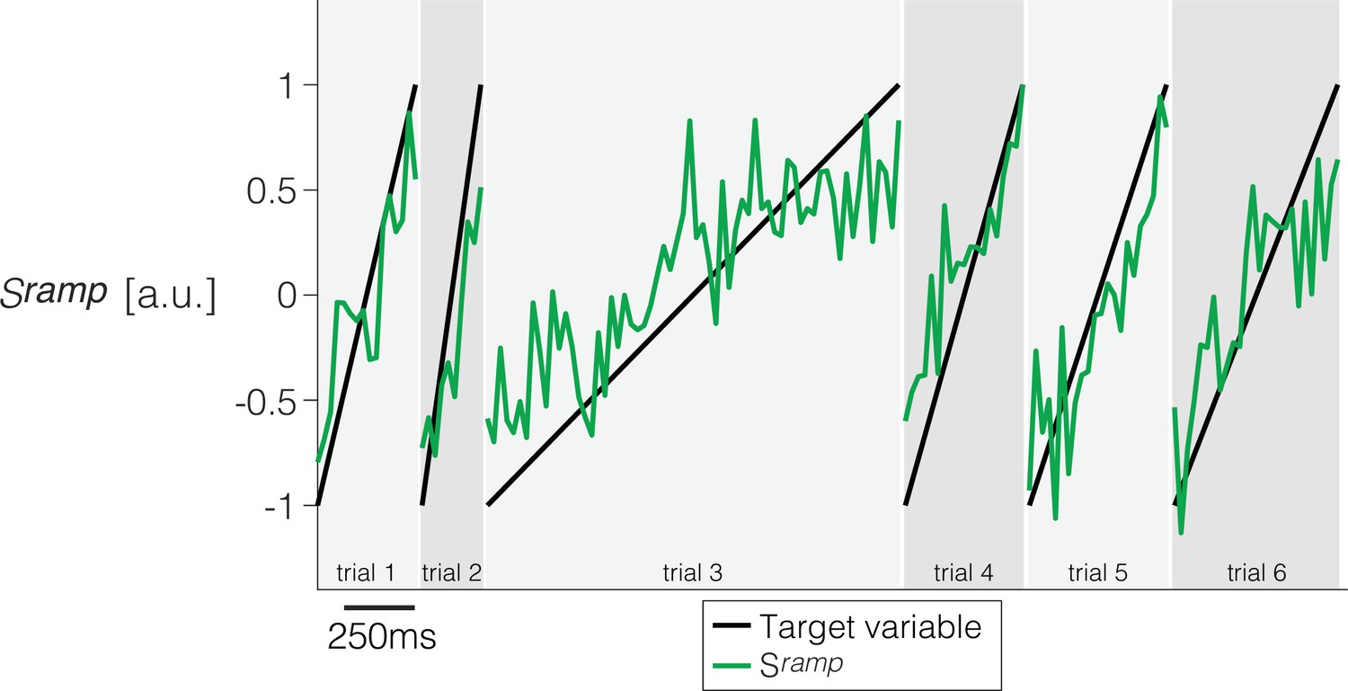
Derivation of a ramp coding direction in neuronal state space.
Weights are assigned to each of the simultaneously recorded neurons in each session using simple least squares regression to approximate a ramp from -1 to +1 on the interval from 200 ms after motion onset to 100 ms before saccade initiation. Only trials ending in left (contraversive) choices are included. The graph shows the quality of the regression on six trials from Session 1. Projection of the population firing rates on the vector of weights renders the single-trial signal, .
Figure 2—figure supplement 2

Trial-averaged activity grouped by reaction time (RT) quantile.
Rows show the averages of single-trial responses of three signals. Choice and RT quantile are indicated by color (legend) and aligned to motion onset (left) and saccade initiation (right). (a) Ramp coding direction. (b) First principal component from principal component analysis (PCA). (c) Averages of the subset of neurons that have the left (contralateral) target in their response field. Correct and error trials are included in both motion and saccade aligned averages.
Figure 2—figure supplement 3
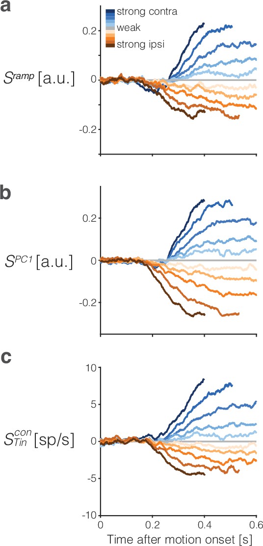
Trial-averaged activity after subtracting the urgency component.
The urgency signal, , is a time-dependent, evidence-independent component of the neural activity that is thought to implement the equivalent of a collapsing bound in the race model architecture of drift-diffusion shown in (Figure 1c). We estimate for each signal, , as the average , aligned to motion onset, using only the 0% coherence motion trials (gray traces in the third column of Figure 2). (a) Ramp coding signal, , with urgency subtracted. (b) PC1 signal with urgency subtracted. (c) signal with urgency subtracted.
Figure 3 with 1 supplement

Variance and autocorrelation of the single-trial signals.
The analyses here are based on samples of at six time points during the first 300 ms of putative integration, using all 0% and ±3.2% coherence trials (). Samples are separated by the width of the boxcar filter (51 ms), beginning at ms. (a) Variance increases as a function of time. The measure of variance is normalized so that it is 1 for the first sample. Error bars are s.e. (bootstrap). (b) Autocorrelation of samples as a function of time and lag approximate the values expected from diffusion. The upper triangular portion of the 6 × 6 correlation matrix for unbounded diffusion ( is represented by brightness). The values from the data () are similar (right). (c) Nine of the 15 autocorrelation terms in (b) permit a more direct comparison of theory and data. The lower limb of the C-shaped function shows the decay in as a function of lag (). This is the top row of (b). The upper limb shows the increase in as a function of time (for fixed lag). This is the lower diagonal in (b). Error bars are s.e. (bootstrap). Note that the autocorrelations incorporate a free parameter, , that serves to correct for an unknown fraction of the measured variance that is not explained by diffusion (see ‘Methods’).
Figure 3—figure supplement 1

Bounds induce sublinear increase in variance of diffusion paths.
For unbounded diffusion (black), the variance across diffusion paths increases linearly with unity slope, and this holds under our smoothing procedure too. Symbols mark the median sample times of the first six non-overlapping ms running means from the beginning of the epoch of integration, as in Figure 3a. The red trace shows the values produced by simulating the model illustrated in Figure 1c (combined residuals from 20,000 trials per coherence –.032, 0, and +.032, as in Figure 3a).
Figure 4 with 5 supplements

The population signal predictive of choice and reaction time (RT) is approximately one-dimensional.
Two binary decoders were trained to predict the choice (What-decoder) and its time (When-decoder) using the population responses in each session. The When-decoder predicts whether a saccadic response to the contralateral target will occur in the next 150 ms, but critically, its accuracy is evaluated based on its ability to predict choice. (a) Cross-validated choice decoding accuracy plotted as a function of time from motion onset (left) and time to saccadic choice (right). Values are averages across sessions. The What-decoder is either trained at the time point at which it is evaluated (time-dependent decoder, orange) or at the single time point indicated by the red arrow ( ms after motion onset; fixed training-time decoder, red). Both training procedures achieve high levels of accuracy. The When-decoder is trained to capture the time of response only on trials terminating with a left (contraversive) choice. The coding direction identified by this approach nonetheless predicts choice (green) nearly as well as the fixed training-time What-decoder. The black trace shows the accuracy of a What-decoder trained on simulated signals using a drift-diffusion model that approximates the behavioral data in Figure 1. Error bars signify s.e.m. across sessions. The gray bar shows the epoch depicted in the next panel. (b) The heat map shows the accuracy of a decoder trained at times along the abscissa and tested at times along the ordinate. Time is relative to motion onset (gray shading in a). In addition to training at ms, the decoder can be trained at any time from ms (dashed box) and achieve the same level of accuracy when tested at any single test time. The orange and red traces in a correspond to the main diagonal () and the column marked by the red arrow, respectively. (c) Trial-averaged activity rendered by the projection of the population responses along the When coding direction, . Same conventions as in Figure 2. (d) Cosine similarity of five coding directions. The heatmap shows the mean values across the sessions, arranged like the lower triangular portion of a correlation matrix. Cosine similarities are significantly greater than zero for all comparisons (all , t-test). (e) Correlation of single-trial diffusion traces. The Pearson correlations are calculated from ordered pairs of , where are the detrended signals rendered by coding directions, and , on trial . The detrending removes trial-averaged means for each signed coherence, leaving only the diffusion component. Reported correlations are significantly greater than zero for all pairs of coding directions and sessions (all , t-test, see ‘Methods’). The variability in cosine similarity and within-trial correlation across sessions is portrayed in Figure 4—figure supplement 3.
Figure 4—figure supplement 1
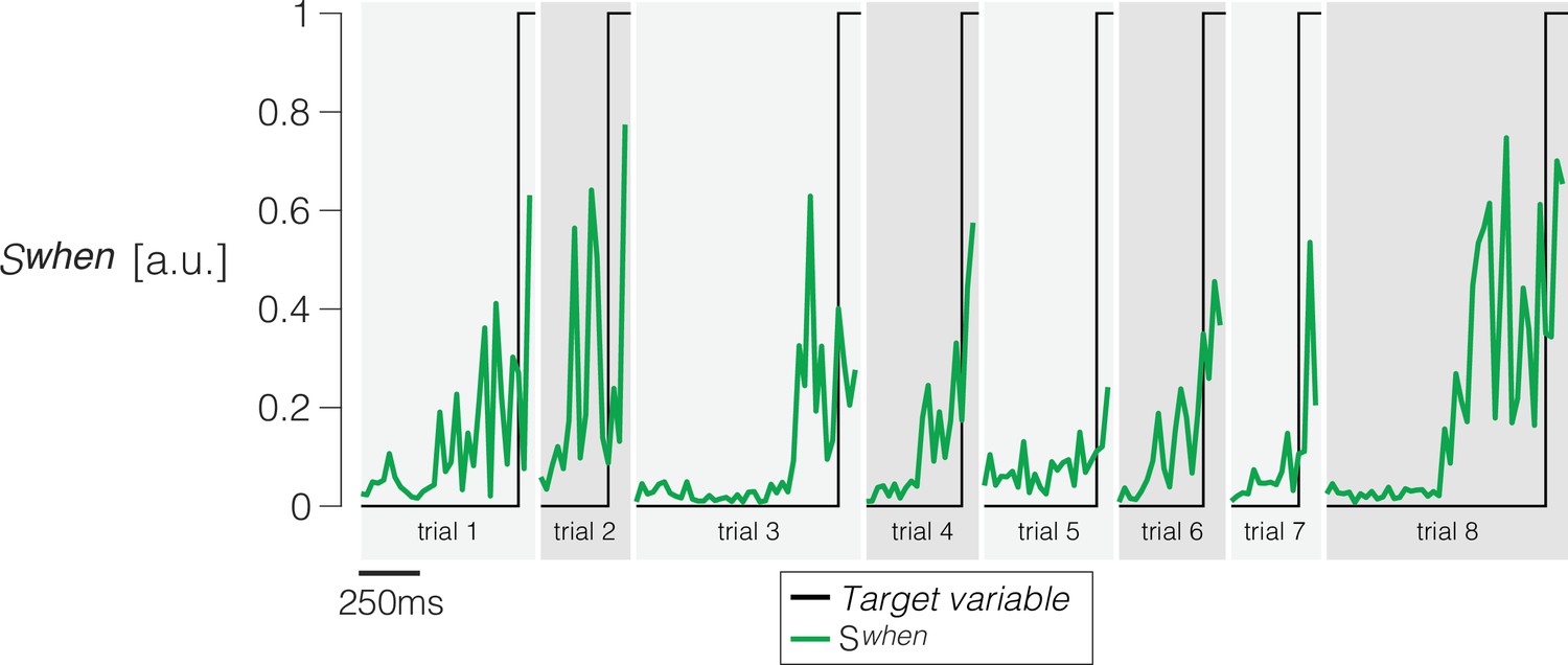
Weights are assigned to each of the simultaneously recorded neurons in each session using logistic regression to approximate a step that takes a value of 0 from 200 ms before motion onset to 150 ms before saccade initiation, and a value of 1 for the following 100 ms (the last 50 ms before the saccade are discarded).
Only trials ending in left (contraversive) choices are included. The graph shows the quality of the regression on eight example trials. The traces are shown from 200 ms after motion onset to 50 ms before the saccade. Projection of the population firing rates on the vector of weights renders the single-trial signal, .
Figure 4—figure supplement 2
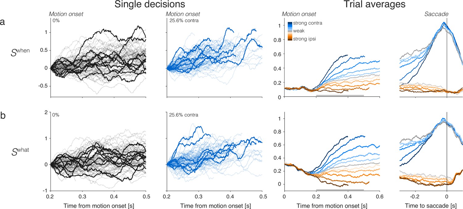
Single-trials and trial-averaged signals furnished by the When- and What-decoders.
Same convention as Figure 2, using the same single-trial examples.
Figure 4—figure supplement 3
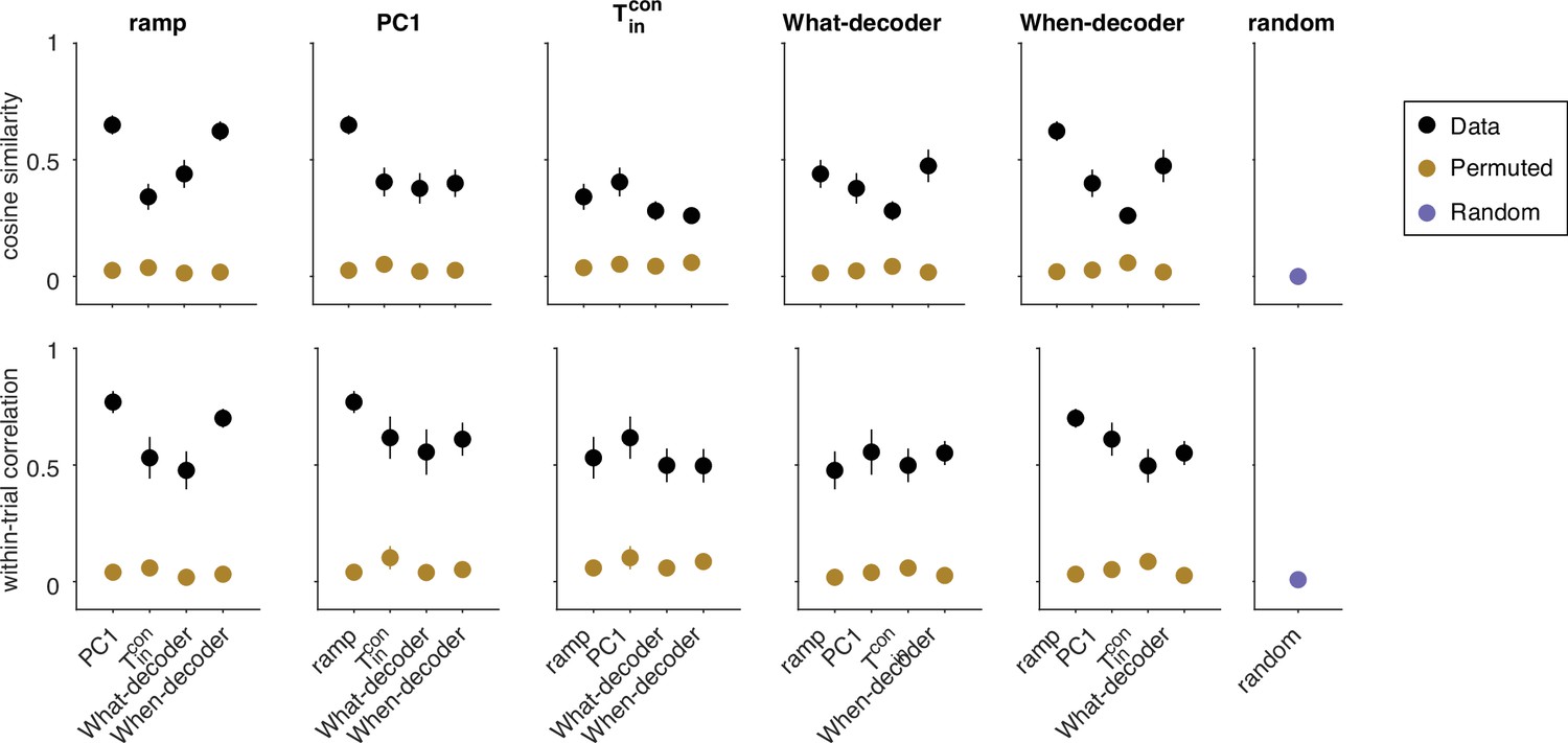
Variability in cosine similarity and within-trial correlation across sessions.
Top. Cosine similarity (CS) of five coding directions. Black markers portray the same mean CS as in Figure 4d. Here, we also show the variability in each measure across sessions (s.e.m.). CS are significantly greater than zero between all pairs of CDs (all p<0.001, t-test). Brown markers portray the same measure when the assignment between neurons and weights are permuted. Error bars reflect the standard deviation across 1000 such permutations. The purple marker in the rightmost column reflects the CS between random directions in state space. These vectors were generated by drawing from a normal distribution, and scaled to length 1. The CS in the data (black symbols) are significantly greater than the CS obtained from the two control analyses, for every pairwise combination of coding directions (permuted weights: all , t-test; random unit vectors: all ). Bottom. Same conventions as top for the within-trial correlations portrayed in Figure 4e. For each pair of coding directions, the within-trial correlations in the data are significantly greater than zero (all ). The correlations are also significantly greater than those between pairs of signals generated by projections of the data onto pairs of (i) random vectors established by permutations of the weights defining each coding direction (brown, all pairwise comparisons , z-test) and (ii) random unit vectors (purple, all pairwise comparisons , z-test). This control serves mainly to refute the possibility that the correlations are explained by correlated variability in the neural population regardless of the signals produced by the weighted sums.
Figure 4—figure supplement 4
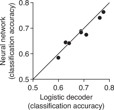
Comparison of linear and non-linear choice decoders.
The figure depicts the cross-validated classification accuracy of two decoders that use population activity at ms from motion onset to predict choice at the same time point on held out trials. The first is a linear decoder (logistic classifier, abscissa), as used for the What decoder in Figure 4. The second is a non-linear decoder (ordinate), which takes the form of a neural network with two hidden layers (, units with sigmoid activation function). The two decoders perform similarly, with the Neural network outperforming the logistic decoder in only one of eight sessions. The analysis suggests that the assumption of linear embedding of the DV is justified.
Figure 4—figure supplement 5

Decoding choice from subsets of neurons.
Mean accuracy (across sessions) of four choice decoders, plotted as a function of time from motion onset (left) and time to saccadic choice (right). The decoders are trained on the neural activity between 425 and 475 ms from motion onset (gray arrow) and applied to all other time points (same method as Figure 4a, fixed training-time). Colors indicate whether the decoders were trained using the activity of all neurons (red, same as in Figure 4a), only and neurons (yellow), all but neurons (purple), or all but and neurons (blue). Decoding accuracy is diminished without the contribution of neurons, which constitute only of the population (mean ± s.e.)
Figure 5 with 3 supplements

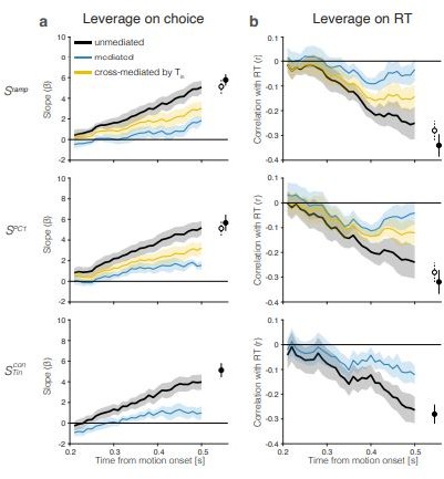
The drift-diffusion signal approximates the decision variable.
The graphs show the leverage of single-trial drift-diffusion signals on choice and reaction time (RT) using only trials with s. Rows correspond to the same coding directions as in Figure 2. The graphs also demonstrate a reduction of the leverage of the samples at s by a later sample of the signal at s. Error bars are s.e.m. across sessions. (a) Leverage of single-trial drift-diffusion signals on choice. Leverage is the value of , the coefficient that multiplies in Equation 8. The black traces show the increase in leverage as a function of time. The dashed linestyle at the left end of three of the traces indicate values that are not statistically significant (p>0.05, bootstrap shuffle test, see ‘Methods’). Filled symbols show the leverage at s. The blue curve (mediated) shows the leverage when the later sample is included in the regression (Equation 9). Open symbols show the leverage of at s (same value as the filled symbol in bottom row). The yellow curves (top and middle rows) show the leverage of the cross-mediated signal by . For all three signals, , leverage at t = 0.4 s is significantly mediated by and cross-mediated by (all , paired samples t-test). (b) Leverage of single-trial drift-diffusion signals on response time. Same conventions as in (a). Leverage is the correlation between and RT. The mediated leverage is the partial correlation, given the later sample. For all three signals, , leverage at t = 0.4 s is significantly mediated by and cross-mediated by (all , paired samples t-test).
Figure 5—figure supplement 1

Control analyses bearing on the leverage and mediation results in Figure 5.
(a) Leverage of signals generated by projection of the neural data on random coding directions in neuronal state space (permutations of the PC1 weights). Same conventions and ordinate scale as in Figure 5. (b) Leverage of drift-diffusion signals derived from simulations of the racing drift-diffusion model fit to behavior (Figure 1). The simulated signals establish the expectation of weakly correlated noisy neurons. The traces agree qualitatively with the leverage and degree of mediation by neurons. Importantly, these simulations highlight that the mediation of the leverage on behavior by a later sample is not complete unless the system is noise-free (for more details see ‘Leverage of single-trial activity on behavior’). Same conventions as in Figure 5.
Figure 5—figure supplement 2
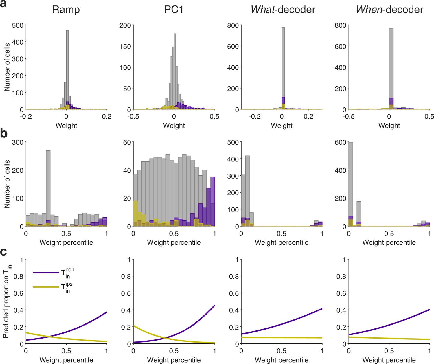
The neurons are not discoverable by their weight assignments.
The neurons contribute strongly and positively to all coding directions, but they are a small fraction of the sampled population. Here we ask whether the rank of a neuron’s weight might identify it as . (a) Distribution of weights assigned to (purple), (yellow) and all other neurons (gray) for the coding directions specified by the column title. (b) Same as (a) for weight percentiles (computed within session). (c) The graphs are logistic fits, where if neuron is , and otherwise. Neurons with stronger positive or negative weights are more likely to be or , respectively, but even the largest weight percentile identifies a neuron with probability less than 0.4.
Figure 5—figure supplement 3
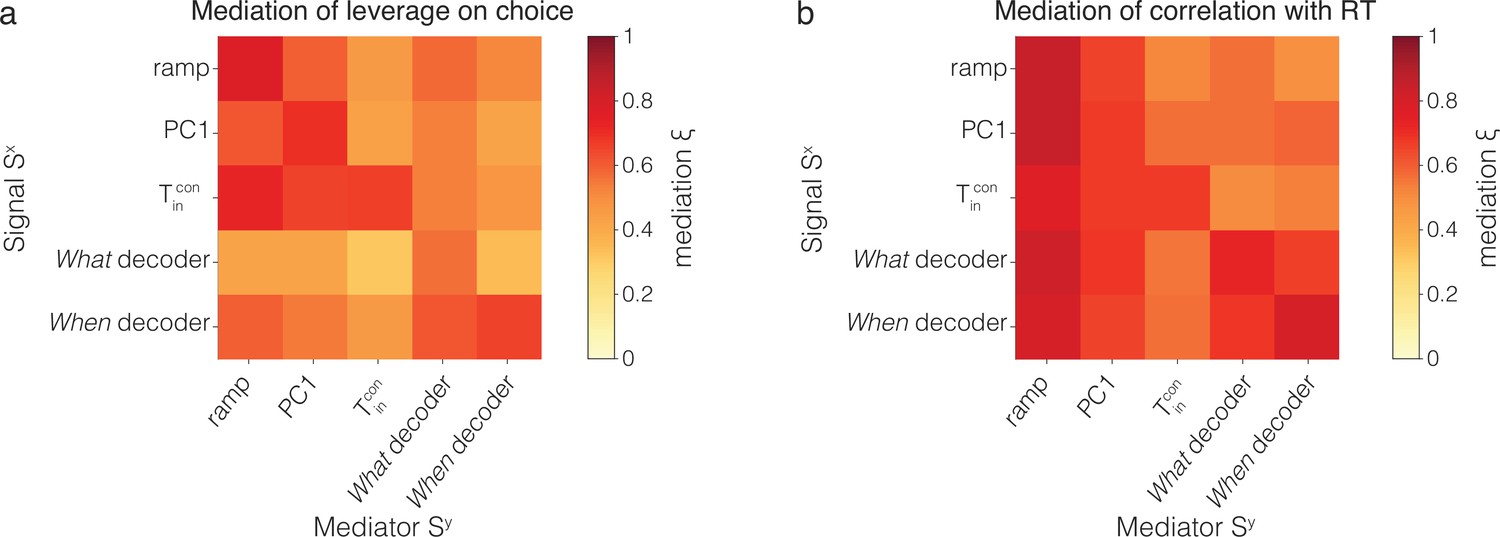
Cross-mediation of single-trial correlations with behavior.
The figure extends the observations in Figure 5 that a sample of at ms after motion onset (i) reduces the leverage of earlier samples of on choice and reaction time (RT) (mediation of on ) and (ii) also reduces the leverage of earlier samples of other signals, and (cross-mediation of on ). The heatmaps are matrices of the mediation indices, and (Equations 10 and 7), that is, how a signal at ms mediates a signal at ms after motion onset. The index is zero if there is no mediation by the later sample; one of the mediation is complete. The main diagonal (top left to bottom right) shows the mediation of (0.55) on (0.4). Values below the diagonal show cross-mediation of by ; values above the diagonal show mediation of by . (a) Leverage on choice. (b) Leverage on RT. Notice that the matrices are not symmetric. For example, mediates the leverage of on choice more mediates the leverage of , and mediates the leverage of on RT more than mediates the leverage of .
Figure 6
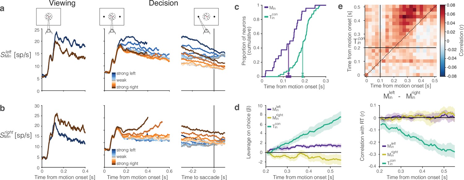
The representation of momentary evidence in area lateral intraparietal cortex (LIP).
(a) Leftward preferring neurons. Left, response to strong leftward (blue) and rightward (brown) motion during passive viewing. Traces are averages over neurons and trials. The neurons were selected for analysis based on this task, hence the stronger response to leftward is guaranteed. Note the short-latency visual response to motion onset followed by the direction-selective (DS) response beginning ∼100 ms after motion onset. Right, Responses during decision-making, aligned to motion onset and the saccadic response. Response averages are grouped by direction and strength of motion (color legend). The neurons retain the same direction preference during passive viewing and decision-making. The responses are also graded as a function of motion strength. (b) Rightward preferring neurons. Same conventions as (a). (c) Cumulative distribution of the times at which individual neurons start showing evidence-dependent activity. Evidence dependence emerges earlier in and neurons (purple) than in neurons (green). Arrows indicate the mean onset of evidence-dependent activity in each signal. The markers at the end of the arrows show the s.e.m. across neurons. (d) Left, leverage of neural activity on choice for (green), (purple), and (yellow) neurons.Rright, same as left, for the correlation between neural activity and reaction time. The absence of negative correlation is explained by insufficient power (see ‘Methods’). (e) Correlation between the neural representation of motion evidence—the difference in activity of neurons selective for leftward and rightward motion —and the neural representation of the decision variable across different time points and lags. Horizontal and vertical lines indicate the onset of evidence-dependent activity in each signal. Positive correlations in the upper-left triangle indicate that the decision variable at a time point is correlated with earlier activity of the evidence signal.
Author response image 1

Shuffle control for Fig.5.
Breaking the within-trial correspondence between neural signal, 𝑆(𝑡), and choice suppresses leverage to near zero.
Author response image 2

Leverage of the integrated difference signal on choice and RT.
Traces are the average leverage across seven sessions. Same conventions as in Figure 5.
Author response image 3

Trial-averaged 𝑆ramp activity during individual sessions.
Same as Figure 2b for individual sessions for Monkey M (left) and Monkey J (right). The figure is intended to illustrate the consistency and heterogeneity of the averaged signals. For example, the saccade-aligned averages lose their association with motion strength before left (contra) choices in sessions 1, 2, 5, and 6 but retain the association in sessions 3, 4, 7, and 8.
Author response image 4
Drift-diffusion signals have measurable leverage on choice and RT even when only 0%-coherence trials are included in the analysis.
Author response image 5

Raw single-trial activity for three types of population averages.
Representative single-trial activity during the first 300 ms of evidence accumulation using two motion strengths: 0% and 25.6% coherence toward the left (contralateral) choice target. Unlike in Figure 2 in the paper, single-trial traces are not baseline corrected by subtracting the activity in a 50 ms window around 200 ms. We highlight a number of trials with thick traces and these are the same trials in each of the rows.
Tables
Table 1
Information about individual experimental sessions.
| Session | 1 | 2 | 3 | 4 | 5 | 6 | 7 | 8 | Mean |
|---|---|---|---|---|---|---|---|---|---|
| Monkey | M | M | M | M | M | J | J | J | |
| Trials | 1797 | 1696 | 2256 | 1859 | 2076 | 2449 | 2799 | 2894 | 2228 |
| Neurons | 191 | 90 | 54 | 140 | 107 | 138 | 161 | 203 | 135.5 |
| % | 8.9 | 14.4 | 16.7 | 15 | 17.8 | 8.7 | 21.1 | 13.3 | 14.5 |
| % | 4.2 | 5.6 | 13 | 13.6 | 6.5 | 12.3 | 0.6 | 2.0 | 7.2 |
| % | 5.2 | 5.6 | 0 | 5 | 3.7 | 2.9 | 3.7 | 7.4 | 4.2 |
| % | 1.0 | 2.2 | 3.7 | 1.4 | 2.8 | 3.6 | 2.5 | 3.0 | 2.5 |
Table 2
Model fit parameters.
κ: scaling of motion strength to drift rate; : bound height; : linear urgency component; : mean of the non-decision time; : standard deviation of the non-decision time; and : bias.
| Parameter | ||||||
|---|---|---|---|---|---|---|
| Monkey M | 13.37 | 1.03 | 0.4199 | 0.317 | 0.039 | –0.0144 |
| Monkey J | 13.72 | 1.76 | 1.3591 | 0.291 | 0.055 | 0.0008 |
Author response table 1
Mean weights assigned to neuron classes in four coding directions.
| Neuron class | Sramp | SPC1 | SWhen | SWhat |
|---|---|---|---|---|
| wTinC | 0.073 | 0.093 | 0.063 | 0.059 |
| wTinI | -0.035 | -0.063 | -0.027 | -0.022 |
| wMinL | 0.011 | 0.012 | 0.028 | 0.027 |
| wMinR | -0.035 | -0.043 | -0.027 | 0.014 |
| wother | 0.0010 | 0.0051 | 0.0020 | 0.0070 |
Additional files
Download links
A two-part list of links to download the article, or parts of the article, in various formats.
Downloads (link to download the article as PDF)
Open citations (links to open the citations from this article in various online reference manager services)
Cite this article (links to download the citations from this article in formats compatible with various reference manager tools)
Direct observation of the neural computations underlying a single decision
eLife 12:RP90859.
https://doi.org/10.7554/eLife.90859.3


