Figures and data in Transformation of valence signaling in a mouse striatopallidal circuit

Version of Record: October 30, 2024 Read the peer reviews
Reviewed Preprint: v3 August 21, 2024
Reviewed Preprint: v2 March 4, 2024
Reviewed Preprint: v1 October 9, 2023

Download
A two-part list of links to download the article, or parts of the article, in various formats.
Downloads (link to download the article as PDF)
- Article PDF
- Figures PDF
Open citations (links to open the citations from this article in various online reference manager services)
- Mendeley
Cite this article (links to download the citations from this article in formats compatible with various reference manager tools)
Donghyung Lee

Nathan Lau

Lillian Liu

Cory M Root

(2024)
Transformation of valence signaling in a mouse striatopallidal circuit

eLife 12:RP90976.

https://doi.org/10.7554/eLife.90976.4
- Download BibTeX
- Download .RIS
Cite
Share
CommentOpen annotations (there are currently 0 annotations on this page).

Figures
Tables
Additional files

6 figures, 59 tables and 1 additional file

Figures

Figure 1 with 1 supplement

Download asset Open asset

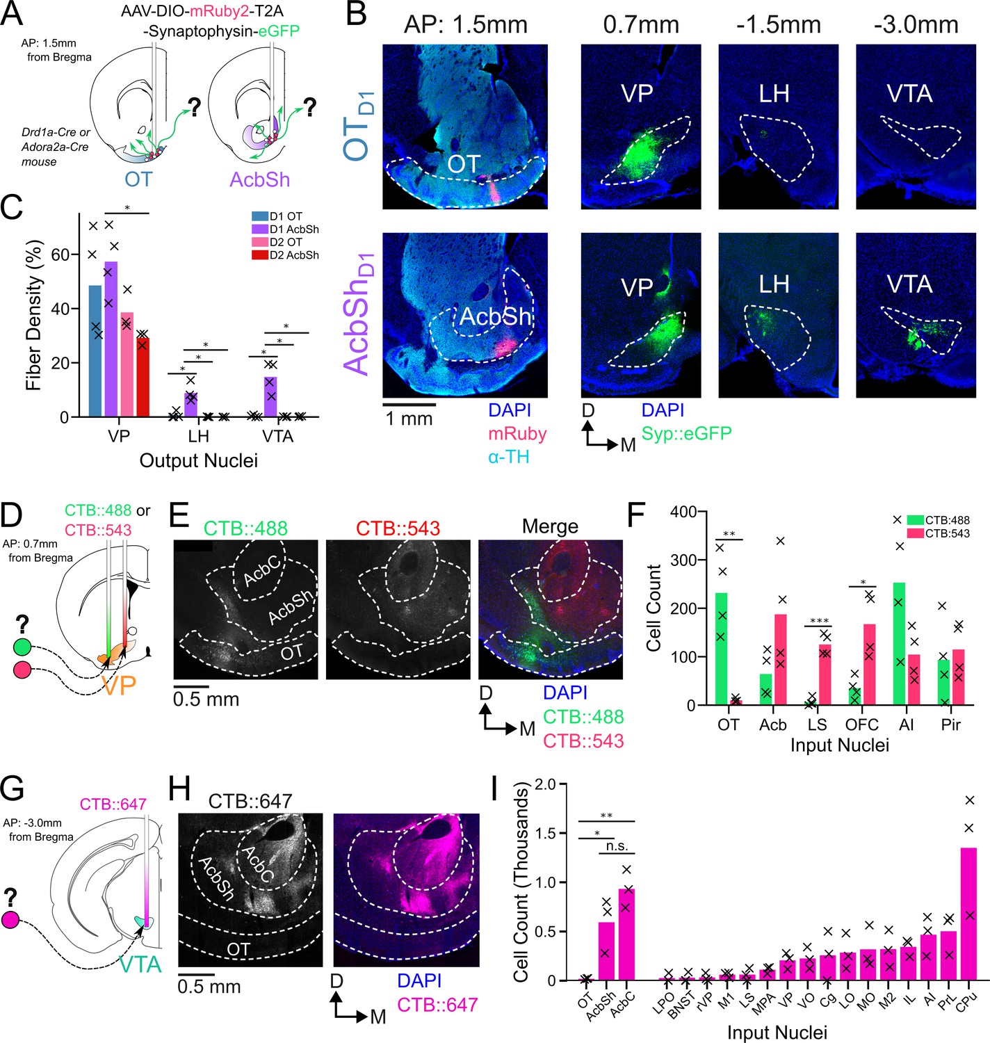
OT_D1 and OT_D2 primarily project to the lateral portion of the VP.

(A) Schematic representation of Cre-dependent anterograde axonal AAV tracing experiments used to characterize outputs of OT neurons. *Drd1+* and *Drd2+* neurons were separately labeled by using *Drd1*-Cre …

Figure 1—figure supplement 1

Download asset Open asset

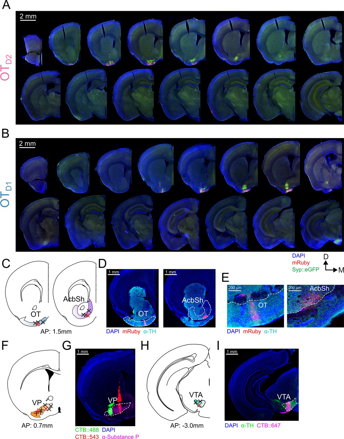
OT_D1 and OT_D2 primarily project to the lateral portion of the VP.

(A) Serial coronal sections from a representative experiment where AAVDJ-hSyn-FLEX-mRuby-T2A-syn-eGFP virus was injected into the anterior OT of an *Adora2a*-Cre mouse. Sections are roughly 400 µm …

Figure 2 with 8 supplements

Download asset Open asset

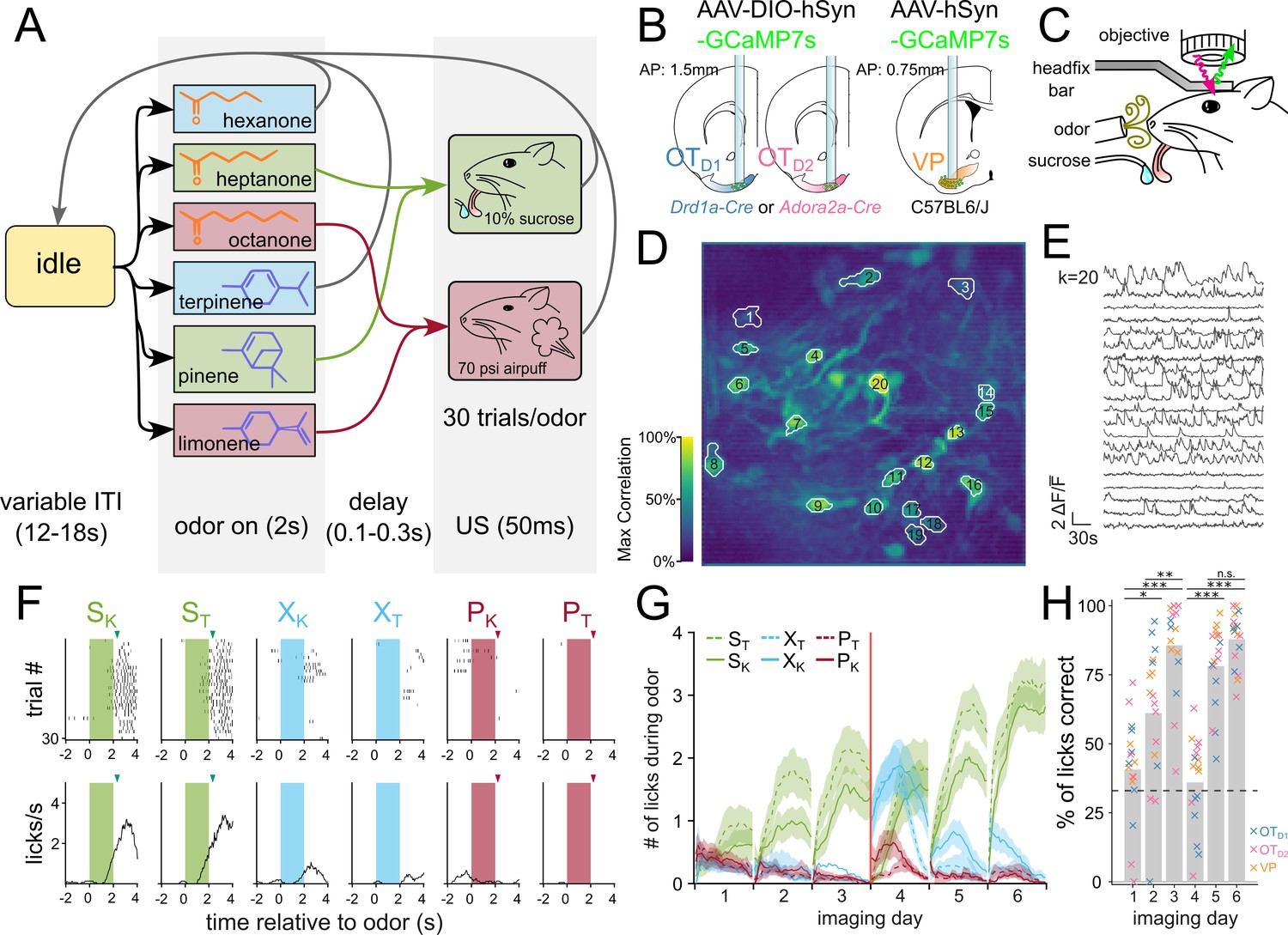
Head-fixed two-photon Ca2²⁺ imaging of OT_D1, OT_D2, or VP neurons during 6-odor conditioning paradigm.

(A) State-diagram of odor conditioning paradigm. Each trial begins with 2 s of odor delivery. Odors are chosen in pseudorandomized order such that the same odor is not repeated more than twice in a …

Figure 2—figure supplement 1

Download asset Open asset

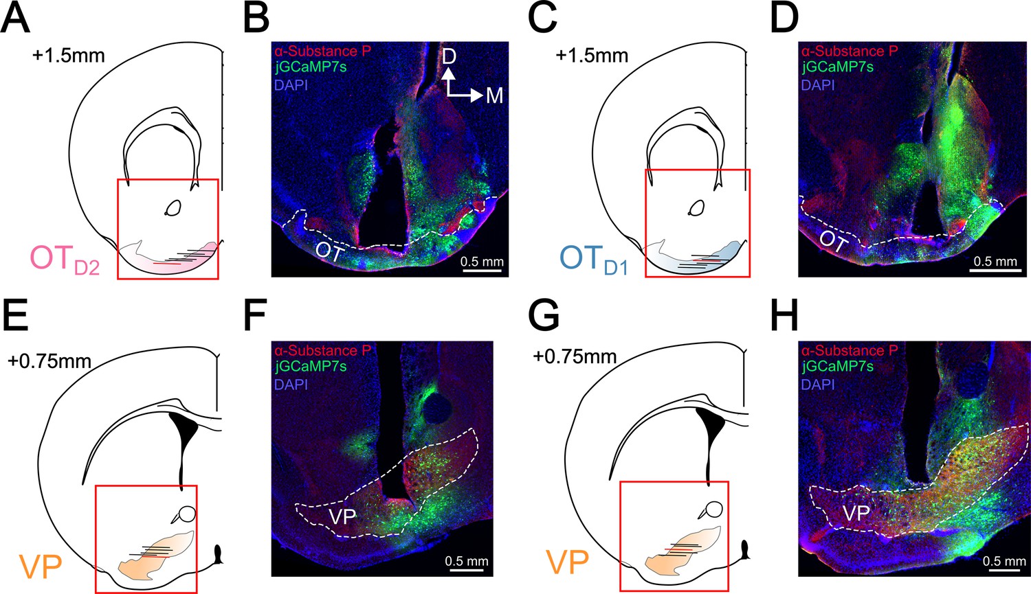
Histological verification of lens implant location.

(A) Schematic showing the center, along the AP axis, of the implanted GRIN lens in six OT_D2 jGCaMP7s animals. (B) Representative image of lens implant sites shown in (A). Sections were …

Figure 2—figure supplement 2

Download asset Open asset

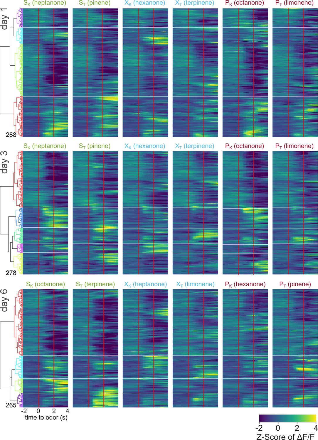
Pooled averaged-over-trials neural activity of all neurons from OT_D2 animals across days.

Heatmap of odor-evoked activity in OT_D2 neurons from day 1, day 3, and day 6 of imaging. The fluorescence measurements from each neuron were averaged over trials, Z-scored, then pooled for …

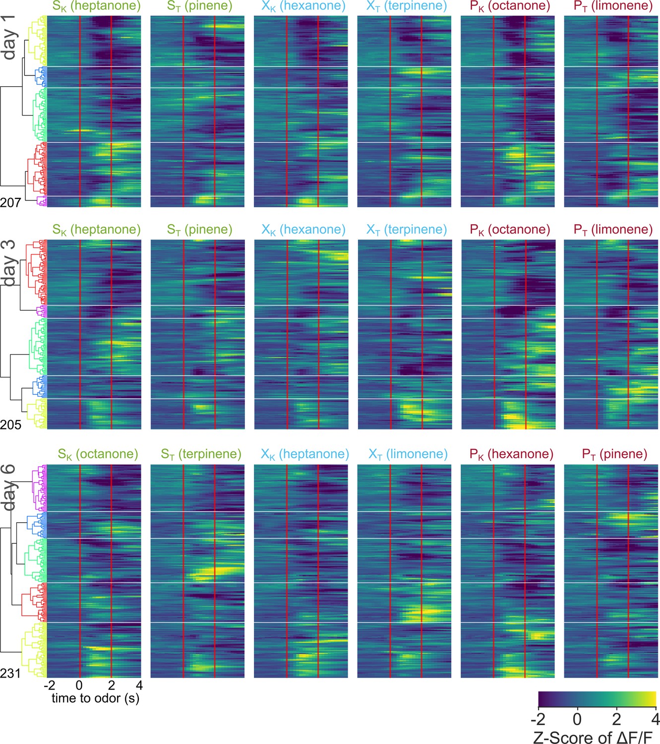
Figure 2—figure supplement 3

Download asset Open asset

Pooled averaged-over-trials neural activity of all neurons from OT_D1 animals across days.

Heatmap of odor-evoked activity in OT_D1 neurons from day 1, day 3, and day 6 of imaging. The fluorescence measurements from each neuron were averaged over trials, Z-scored, then pooled for …

Figure 2—figure supplement 4

Download asset Open asset

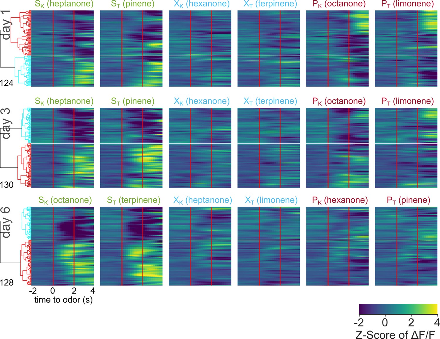
Pooled averaged-over-trials neural activity of all neurons from VP animals across days.

Heatmap of odor-evoked activity in VP neurons from day 1, day 3, and day 6 of imaging. The fluorescence measurements from each neuron were averaged over trials, Z-scored, then pooled for …

Figure 2—figure supplement 5

Download asset Open asset

Extended behavioral analysis from imaging period.

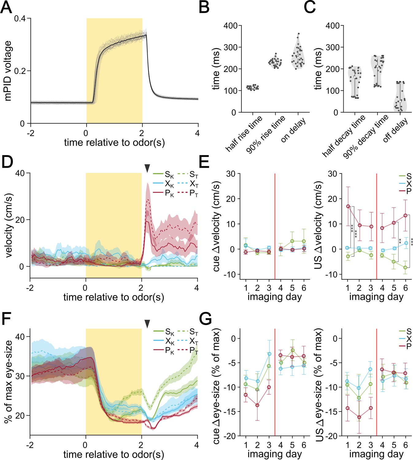
(A) mPID voltage reading in response to 30 trials of a sample odor (α-terpinene) delivery. The time period during which the odor valve was turned on is shown by the yellow rectangle. Individual …

Figure 2—figure supplement 6

Download asset Open asset

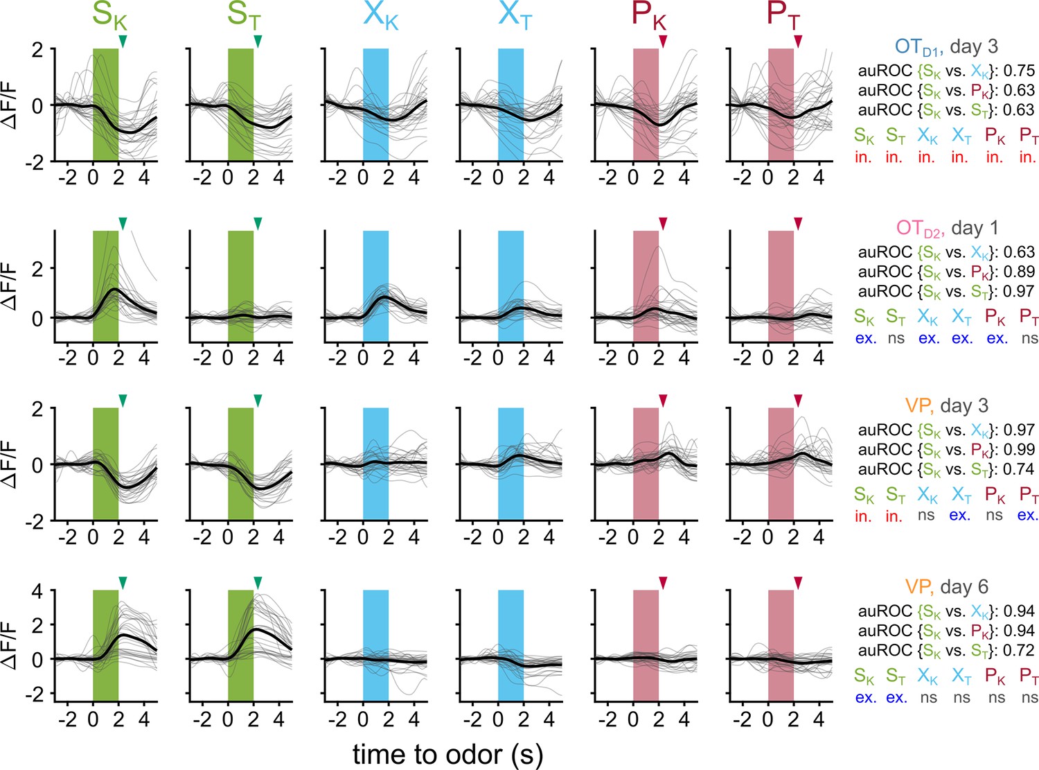
Traces of example neurons and their corresponding metrics.

(A) Example traces from an OT_D1 neuron recorded on day 3. Each column shows this neuron’s response to a given odor across 30 trials (gray). The average across all trials is shown in black. For green …

Figure 2—figure supplement 7

Download asset Open asset

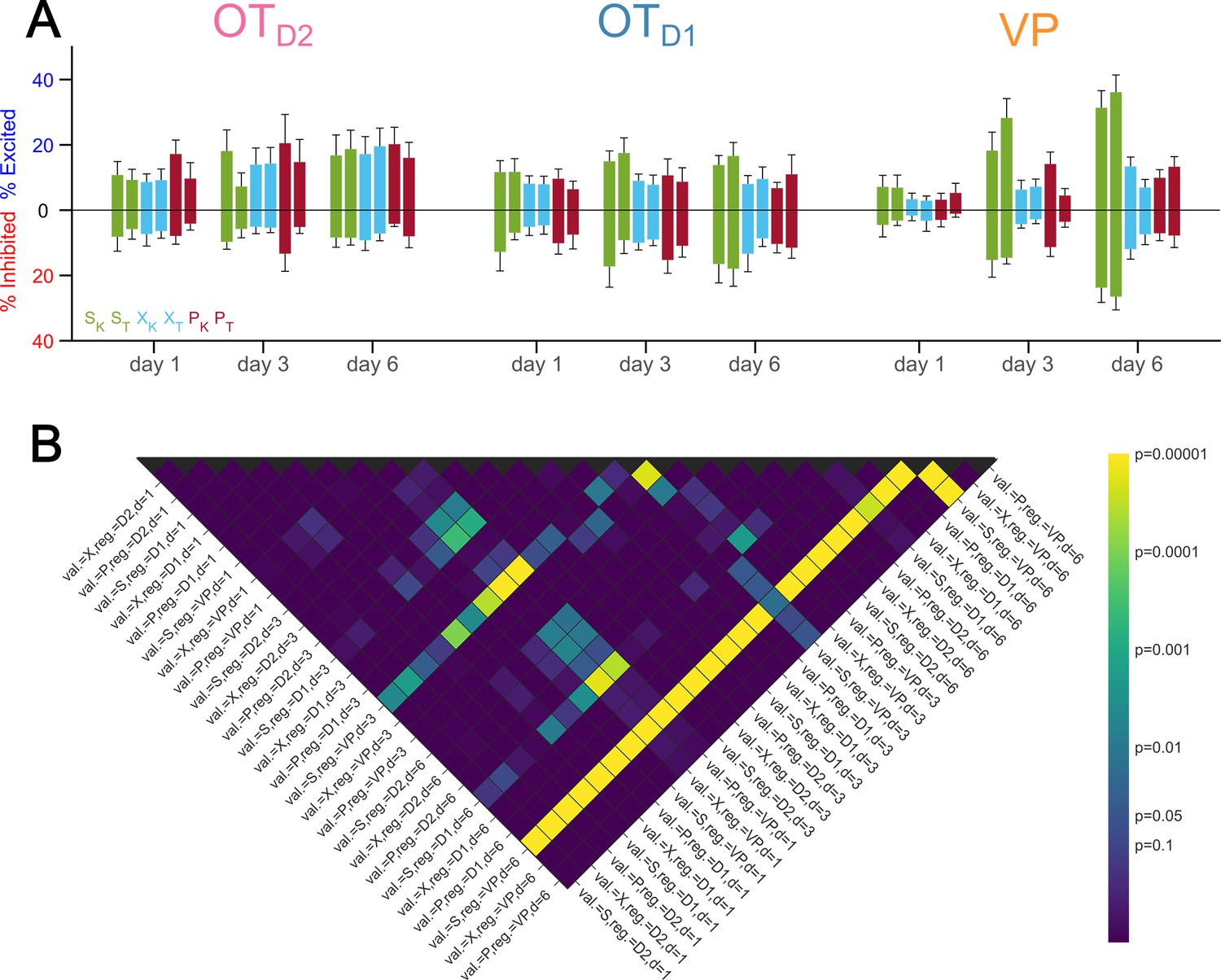
Percentage of neurons responsive to each odor across days.

(A) Bar graphs showing percentage of neurons from each region on imaging days 1, 3, and 6 that were significantly excited or inhibited by each odor. The average across animals is shown by the bar …

Figure 2—figure supplement 8

Download asset Open asset

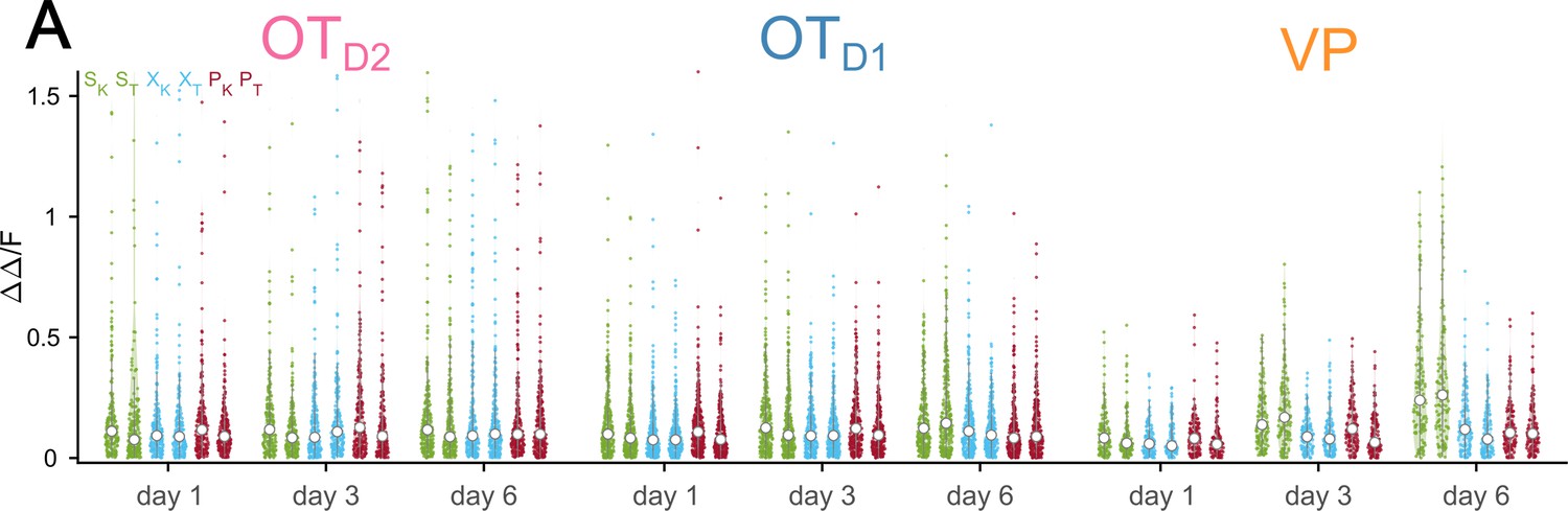
Distribution of response magnitudes to each odor across days.

Violin plots showing the averaged-over-trials response magnitudes to each odor during the last second of odor exposure. See Appendix 1—table 38 for detailed statistics.

Figure 3 with 2 supplements

Download asset Open asset

VP neurons encode reward-contingency more robustly than OT_D1 or OT_D2 neurons.

(A) Heatmap of odor-evoked activities in OT_D1, OT_D2, and VP neurons from day 6 of imaging. The fluorescence measurements from each neuron were averaged over trials, Z-scored, then pooled for …

Figure 3—figure supplement 1

Download asset Open asset

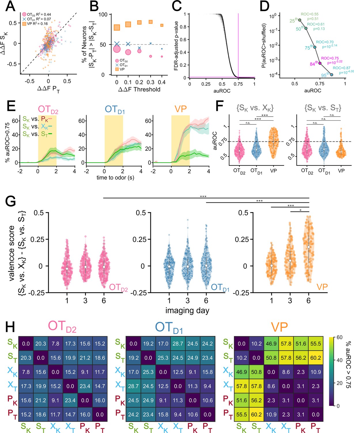
Pairwise analysis of single neuron odor encoding.

(A) Scatterplot comparing the magnitudes of S_K responses (∆∆S_K) to P_T responses (∆∆P_T). The dotted line represents the hypothetical scenario where ∆∆S_K = ∆∆P_T. For each population, the R² value of …

Figure 3—figure supplement 2

Download asset Open asset

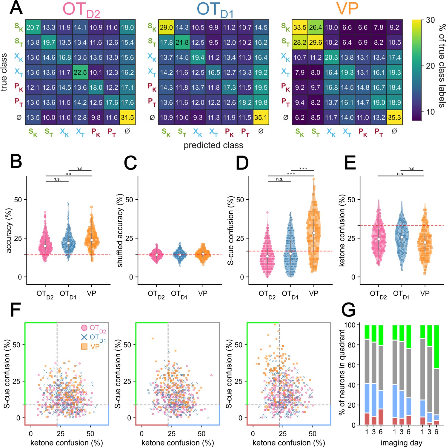
Multinomial analysis of single neuron odor encoding.

(A) Confusion matrix of single-neuron MNR classifiers trained on neural activity during the last second of odor exposure on day 6 of imaging. Rows represent the true class while columns represent …

Figure 4

Download asset Open asset

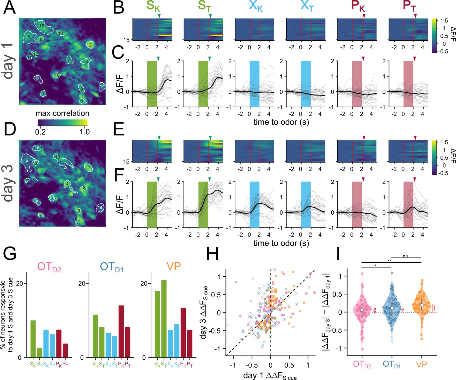
Sucrose responsive VP neurons become sucrose-cue responsive after pairing.

(A) The spatial footprints of 15 neurons from day 1 are outlined over a max-correlation projection image. (B) Heatmap of averaged-over-trials ΔF/F in response to 6 odors on day 1. Odor delivery …

Figure 5 with 1 supplement

Download asset Open asset

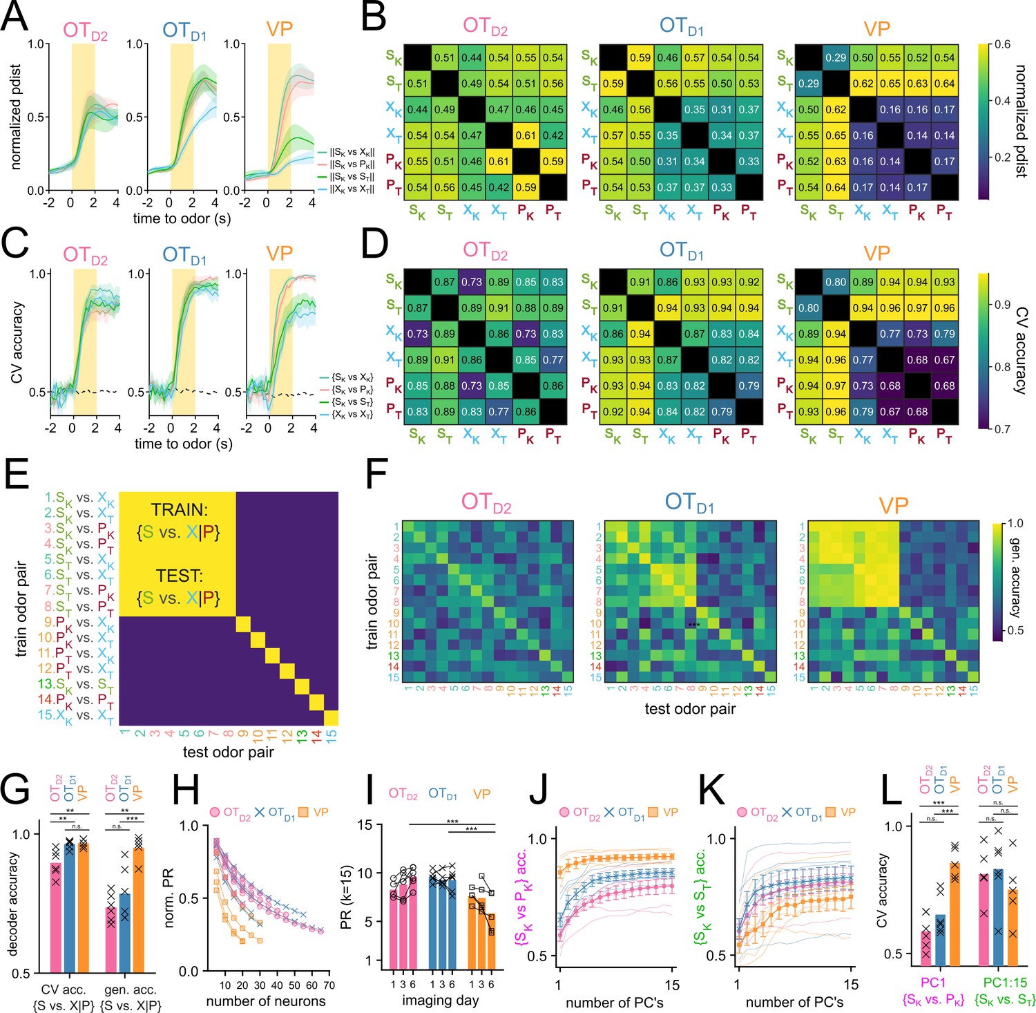
OT encodes odor identity in high-dimensional space and VP encodes reward-contingency in low-dimensional space.

(A) Average normalized pairwise Euclidean distance between odor-evoked population-level activity from day 6 of imaging shown as a function of time relative to odor delivery. Traces show the average …

Figure 5—figure supplement 1

Download asset Open asset

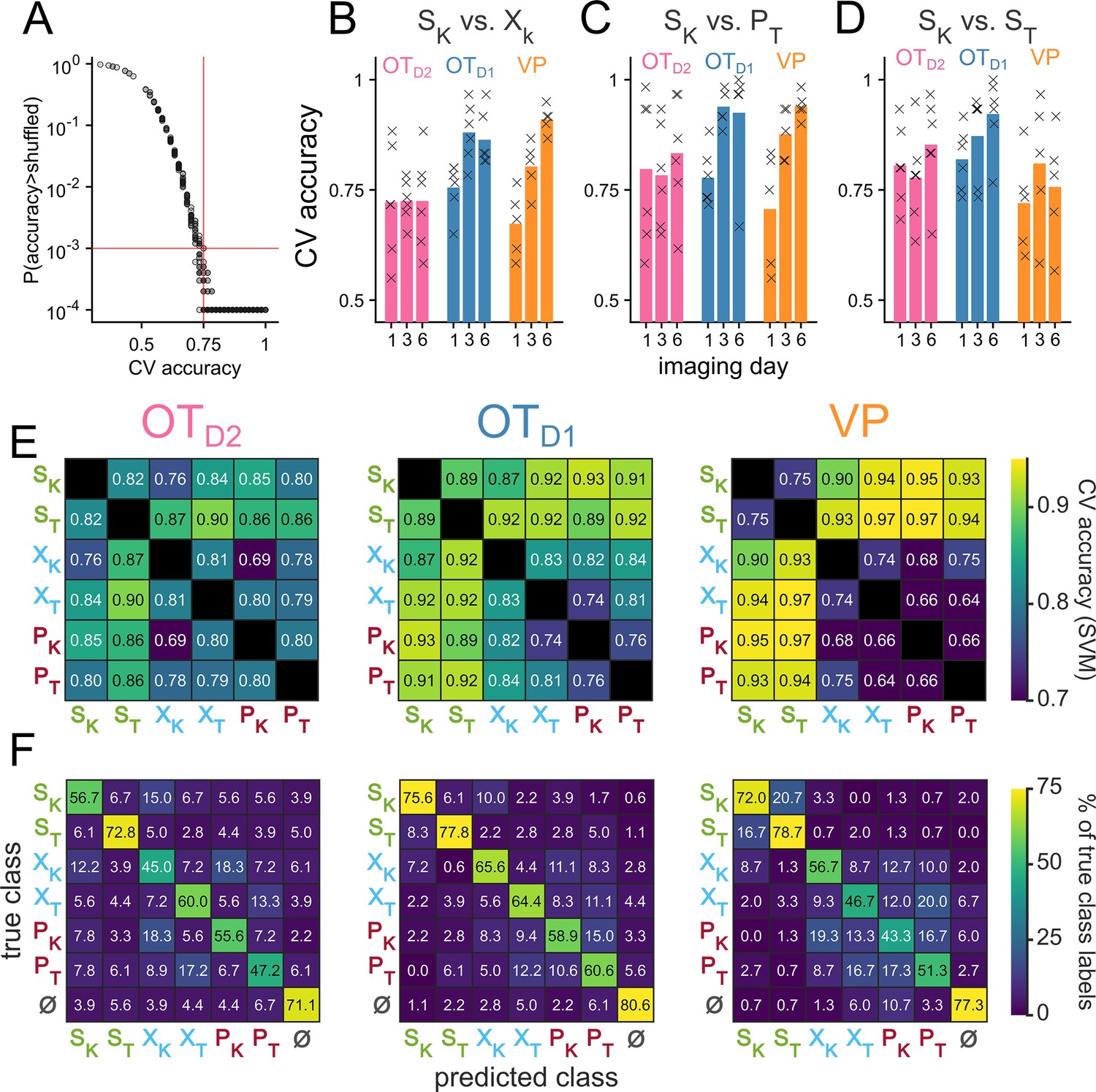
Analysis of population-level odor encoding.

(A) Scatterplot of CV-accuracy of linear classifiers trained on simultaneously-recorded neurons on the x-axis and their bootstrapped unadjusted p-values on the y-axis. Red horizontal line marks …

Figure 6 with 1 supplement

Download asset Open asset

Separate VP populations encode reward-contingency and licking vigor.

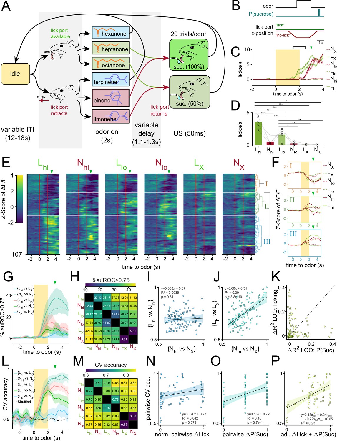
(A) State diagram for odor pairing paradigm where lick spout is removed during the presentation of half of the odors. The paradigm is similar to one described in Figure 2A with the following key …

Figure 6—figure supplement 1

Download asset Open asset

Camera-based detection of licking in head-fixed animals.

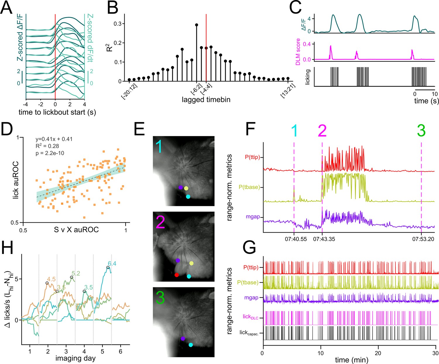
(A–C) Metrics of a representative neurons with activity that predicts licking. (A) Representative neuron’s Z-scored ΔF/F (dark green) and Z-scored dF/dt (light green) aligned to the onset of a …

Tables

Appendix 1—table 1

Pairwise comparisons of anterograde labeling from OT and AcbSh (Figure 1C).

Group A	Group B	Lower Limit	A-B	Upper Limit	FDR adjusted p-value
OT_D1 → VP	Acb_D1 → VP	–20.506	–8.798	2.910	0.577
OT_D1 → VP	OT_D2 → VP	–0.851	9.922	20.694	0.577
OT_D1 → VP	Acb_D2 → VP	9.338	19.340	29.341	0.291
Acb_D1 → VP	OT_D2 → VP	11.163	18.719	26.275	0.161
Acb_D1 → VP	Acb_D2 → VP	21.729	28.137	34.545	3.394E-02
OT_D2 → VP	Acb_D2 → VP	4.942	9.418	13.894	0.206
OT_D1 → VP	Acb_D1 → VP	–9.944	–8.199	–6.453	2.223E-02
OT_D1 → LH	OT_D2 → LH	–0.045	0.564	1.173	0.577
OT_D1 → LH	Acb_D2 → LH	–0.016	0.591	1.198	0.577
Acb_D1 → LH	OT_D2 → LH	7.125	8.763	10.401	2.223E-02
Acb_D1 → LH	Acb_D2 → LH	7.153	8.790	10.426	2.223E-02
OT_D2 → LH	Acb_D2 → LH	–0.029	0.027	0.082	0.655
OT_D1 → VTA	Acb_D1 → VTA	–17.357	–14.504	–11.650	2.223E-02
OT_D1 → VTA	OT_D2 → VTA	–0.022	0.183	0.387	0.577

Appendix 1—table 2

Pairwise comparisons of retrograde labeling from vlVP and dmVP (Figure 1F).

Group A	Group B	Lower Limit	A-B	Upper Limit	FDR adjusted p-value
AI→vlVP	AI→dmVP	78.249	148.500	218.751	0.116
Acb→vlVP	Acb→dmVP	–185.929	–123.250	–60.571	0.116
LS→vlVP	LS→dmVP	–130.496	–118.750	–107.004	3.27E-04
OFC→vlVP	OFC→dmVP	–167.021	–132.000	–96.979	1.86E-02
OT→vlVP	OT→dmVP	179.793	221.750	263.707	5.57E-03
Pir→vlVP	Pir→dmVP	–71.946	–21.500	28.946	0.685

Appendix 1—table 3

Pairwise comparisons of retrograde labeling from VTA (Figure 1I).

Group A	Group B	Lower Limit	A-B	Upper Limit	FDR adjusted p-value
OT→VTA	AcbSh→VTA	–735.101	–575	–414.899	3.44E-02
OT→VTA	AcbC→VTA	–1027.381	–915	–802.619	3.71E-03
AcbC→VTA	AcbSh→VTA	144.452	340	535.548	0.157

Appendix 1—table 4

Two-way ANOVA for effect of day or lens placement on licking accuracy (Figure 2H).

Source	Sum Sq.	d.f.	Mean Sq.	F	Prob >F
day	4.301	5	0.860	27.638	2.29E-16
region	0.143	2	0.072	2.301	0.106
day:region	0.251	10	0.025	0.806	0.623
Error	2.583	83	0.031
Total	7.305	100

Appendix 1—table 5

Post hoc pairwise comparisons of licking accuracy across imaging days (Figure 2H).

Group A	Group B	Lower Limit	A-B	Upper Limit	p-value
day 1	day 2	–0.385	–0.208	–0.031	1.18E-02
day 1	day 3	–0.632	–0.452	–0.272	2.03E-09
day 1	day 4	–0.134	0.043	0.220	0.980
day 1	day 5	–0.558	–0.381	–0.203	2.30E-07
day 1	day 6	–0.650	–0.473	–0.295	2.58E-10
day 2	day 3	–0.424	–0.244	–0.064	2.18E-03
day 2	day 4	0.074	0.251	0.429	1.14E-03
day 2	day 5	–0.350	–0.172	0.005	0.061
day 2	day 6	–0.441	–0.264	–0.087	5.33E-04
day 3	day 4	0.315	0.495	0.675	8.31E-11
day 3	day 5	–0.109	0.071	0.251	0.856
day 3	day 6	–0.200	–0.021	0.159	0.999
day 4	day 5	–0.601	–0.424	–0.247	1.00E-08
day 4	day 6	–0.693	–0.516	–0.338	9.77E-12
day 5	day 6	–0.269	–0.092	0.085	0.657

Appendix 1—table 6

2-way ANOVA for effect of day or lens placement on percentage of neurons responsive to a single odor (Figure 3E).

Source	Sum Sq.	d.f.	Mean Sq.	F	Prob >F
day	0.05917	2	0.02958	2.99563	0.06079
region	0.03696	2	0.01848	1.87142	0.16651
day:region	0.06481	4	0.01620	1.64062	0.18197
Error	0.41479	42	0.00988
Total	0.57170	50

Appendix 1—table 7

Post hoc pairwise comparisons of percentage of neurons responsive to a single odor across imaging days and region (Figure 3E).

Group A	Group B	Lower Limit	A-B	Upper Limit	p-value
d1,D2 OT	d3,D2 OT	–0.140	0.048	0.236	0.995
d1,D2 OT	d6,D2 OT	–0.164	0.024	0.211	1.000
d3,D2 OT	d6,D2 OT	–0.212	–0.024	0.163	1.000
d1,D1 OT	d3,D1 OT	–0.287	–0.099	0.088	0.724
d1,D1 OT	d6,D1 OT	–0.328	–0.141	0.047	0.285
d3,D1 OT	d6,D1 OT	–0.229	–0.041	0.146	0.998
d1,VP	d3,VP	–0.321	–0.115	0.090	0.662
d1,VP	d6,VP	–0.335	–0.129	0.076	0.513
d3,VP	d6,VP	–0.220	–0.014	0.191	1.000
d1,D2 OT	d1,D1 OT	–0.115	0.072	0.260	0.937
d1,D2 OT	d1,VP	–0.056	0.141	0.338	0.341
d1,D1 OT	d1,VP	–0.128	0.069	0.265	0.964
d3,D2 OT	d3,D1 OT	–0.263	–0.075	0.112	0.923
d3,D2 OT	d3,VP	–0.219	–0.022	0.175	1.000
d3,D1 OT	d3,VP	–0.144	0.053	0.250	0.993
d6,D2 OT	d6,D1 OT	–0.280	–0.092	0.095	0.796
d6,D2 OT	d6,VP	–0.209	–0.012	0.184	1.000
d6,D1 OT	d6,VP	–0.117	0.080	0.276	0.918

Appendix 1—table 8

Two-way ANOVA for effect of day or lens placement on percentage of neurons responsive to three or more odors (Figure 3E).

Source	Sum Sq.	d.f.	Mean Sq.	F	Prob >F
day	0.10897	2	0.05448	4.58607	0.01580
region	0.00469	2	0.00234	0.19732	0.82168
day:region	0.06640	4	0.01660	1.39730	0.25144
Error	0.49897	42	0.01188
Total	0.66598	50

Appendix 1—table 9

Post hoc pairwise comparisons of percentage of neurons responsive to three or more odors across imaging days and region (Figure 3E).

Group A	Group B	Lower Limit	A-B	Upper Limit	p-value
d1,D2 OT	d3,D2 OT	–0.237	–0.031	0.175	1.000
d1,D2 OT	d6,D2 OT	–0.246	–0.040	0.165	0.999
d3,D2 OT	d6,D2 OT	–0.215	–0.009	0.196	1.000
d1,D1 OT	d3,D1 OT	–0.230	–0.024	0.182	1.000
d1,D1 OT	d6,D1 OT	–0.269	–0.063	0.143	0.984
d3,D1 OT	d6,D1 OT	–0.245	–0.039	0.167	0.999
d1,VP	d3,VP	–0.406	–0.181	0.044	0.207
d1,VP	d6,VP	–0.453	–0.228	–0.003	0.046
d3,VP	d6,VP	–0.272	–0.047	0.178	0.999
d1,D2 OT	d1,D1 OT	–0.220	–0.014	0.191	1.000
d1,D2 OT	d1,VP	–0.124	0.092	0.308	0.894
d1,D1 OT	d1,VP	–0.109	0.106	0.322	0.793
d3,D2 OT	d3,D1 OT	–0.213	–0.007	0.198	1.000
d3,D2 OT	d3,VP	–0.274	–0.058	0.158	0.993
d3,D1 OT	d3,VP	–0.266	–0.051	0.165	0.997
d6,D2 OT	d6,D1 OT	–0.243	–0.037	0.168	1.000
d6,D2 OT	d6,VP	–0.311	–0.096	0.120	0.871
d6,D1 OT	d6,VP	–0.274	–0.059	0.157	0.993

Appendix 1—table 10

Two-way ANOVA for effect of day or lens placement on percentage of neurons responsive to both S-cues (Figure 3E).

Source	Sum Sq.	d.f.	Mean Sq.	F	Prob >F
day	0.11460	2	0.05730	6.60475	0.00321
region	0.18370	2	0.09185	10.58706	0.00019
day:region	0.16522	4	0.04131	4.76096	0.00294
Error	0.36438	42	0.00868
Total	0.80767	50

Appendix 1—table 11

Post hoc pairwise comparisons of percentage of neurons responsive to both S-cues across imaging days and region (Figure 3E).

Group A	Group B	Lower Limit	A-B	Upper Limit	p-value
d1,D2 OT	d3,D2 OT	–0.139	0.037	0.213	0.999
d1,D2 OT	d6,D2 OT	–0.200	–0.024	0.151	1.000
d3,D2 OT	d6,D2 OT	–0.237	–0.062	0.114	0.963
d1,D1 OT	d3,D1 OT	–0.239	–0.063	0.112	0.957
d1,D1 OT	d6,D1 OT	–0.196	–0.020	0.156	1.000
d3,D1 OT	d6,D1 OT	–0.133	0.043	0.219	0.996
d1,VP	d3,VP	–0.441	–0.248	–0.056	3.79E-03
d1,VP	d6,VP	–0.473	–0.281	–0.088	7.12E-04
d3,VP	d6,VP	–0.225	–0.032	0.160	1.000
d1,D2 OT	d1,D1 OT	–0.189	–0.013	0.163	1.000
d1,D2 OT	d1,VP	–0.151	0.033	0.217	1.000
d1,D1 OT	d1,VP	–0.138	0.046	0.230	0.996
d3,D2 OT	d3,D1 OT	–0.289	–0.114	0.062	0.480
d3,D2 OT	d3,VP	–0.437	–0.252	–0.068	1.72E-03
d3,D1 OT	d3,VP	–0.323	–0.139	0.045	0.279
d6,D2 OT	d6,D1 OT	–0.185	–0.009	0.167	1.000
d6,D2 OT	d6,VP	–0.408	–0.223	–0.039	7.94E-03
d6,D1 OT	d6,VP	–0.399	–0.214	–0.030	1.23E-02

Appendix 1—table 12

Two-way ANOVA for effect of day or lens placement on percentage of neurons with auROC >0.75 for {S_K vs. P_K} (Figure 3I).

Source	Sum Sq.	d.f.	Mean Sq.	F	Prob >F
day	0.85429	2	0.42714	46.23443	2.439E-11
region	0.32224	2	0.16112	17.43954	3.064E-06
day:region	0.40111	4	0.10028	10.85411	3.918E-06
Error	0.38802	42	0.00924
Total	1.87808	50

Appendix 1—table 13

Post hoc comparisons of percentage of neurons with auROC >0.75 for {S_K vs. P_K} across imaging day and region (Figure 3I).

Group A	Group B	Lower Limit	A-B	Upper Limit	p-value
d1,D2 OT	d3,D2 OT	–0.259	–0.078	0.103	0.890
d1,D2 OT	d6,D2 OT	–0.279	–0.097	0.084	0.709
d3,D2 OT	d6,D2 OT	–0.201	–0.020	0.162	1.000
d1,D1 OT	d3,D1 OT	–0.293	–0.112	0.069	0.541
d1,D1 OT	d6,D1 OT	–0.417	–0.236	–0.054	0.003
d3,D1 OT	d6,D1 OT	–0.305	–0.124	0.058	0.407
d1,VP	d3,VP	–0.476	–0.278	–0.079	0.001
d1,VP	d6,VP	–0.820	–0.621	–0.423	2.00E-11
d3,VP	d6,VP	–0.542	–0.344	–0.145	4.09E-05
d1,D2 OT	d1,D1 OT	–0.170	0.011	0.192	1.000
d1,D2 OT	d1,VP	–0.141	0.049	0.239	0.995
d1,D1 OT	d1,VP	–0.152	0.038	0.228	0.999
d3,D2 OT	d3,D1 OT	–0.204	–0.023	0.158	1.000
d3,D2 OT	d3,VP	–0.341	–0.151	0.039	0.221
d3,D1 OT	d3,VP	–0.318	–0.128	0.062	0.427
d6,D2 OT	d6,D1 OT	–0.309	–0.127	0.054	0.370
d6,D2 OT	d6,VP	–0.665	–0.475	–0.285	1.15E-08
d6,D1 OT	d6,VP	–0.538	–0.348	–0.158	1.43E-05

Appendix 1—table 14

Two-way ANOVA for effect of day or lens placement on percentage of neurons with auROC >0.75 for {S_K vs. X_K} (Figure 3J).

Source	Sum Sq.	d.f.	Mean Sq.	F	Prob >F
day	0.551	2	0.275	28.099	1.794E-08
region	0.377	2	0.188	19.265	1.156E-06
day:region	0.364	4	0.0912	9.310	1.764E-05
Error	0.411	42	0.009
Total	1.637	50

Appendix 1—table 15

Post hoc comparisons of percentage of neurons with auROC >0.75 for {S_K vs. X_K} across imaging day and region (Figure 3J).

Group A	Group B	Lower Limit	A-B	Upper Limit	p-value
d1,D2 OT	d3,D2 OT	–0.189	–0.002	0.184	1.000
d1,D2 OT	d6,D2 OT	–0.238	–0.052	0.135	0.992
d3,D2 OT	d6,D2 OT	–0.236	–0.049	0.137	0.994
d1,D1 OT	d3,D1 OT	–0.313	–0.126	0.061	0.421
d1,D1 OT	d6,D1 OT	–0.356	–0.170	0.017	0.102
d3,D1 OT	d6,D1 OT	–0.230	–0.044	0.143	0.997
d1,VP	d3,VP	–0.454	–0.250	–0.045	7.23E-03
d1,VP	d6,VP	–0.750	–0.545	–0.341	2.05E-09
d3,VP	d6,VP	–0.500	–0.295	–0.091	8.14E-04
d1,D2 OT	d1,D1 OT	–0.219	–0.033	0.154	1.000
d1,D2 OT	d1,VP	–0.163	0.033	0.229	1.000
d1,D1 OT	d1,VP	–0.130	0.066	0.261	0.972
d3,D2 OT	d3,D1 OT	–0.343	–0.156	0.031	0.167
d3,D2 OT	d3,VP	–0.410	–0.214	–0.019	2.26E-02
d3,D1 OT	d3,VP	–0.254	–0.058	0.138	0.987
d6,D2 OT	d6,D1 OT	–0.337	–0.151	0.036	0.204
d6,D2 OT	d6,VP	–0.656	–0.461	–0.265	5.39E-08
d6,D1 OT	d6,VP	–0.506	–0.310	–0.114	1.95E-04

Appendix 1—table 16

Two-way ANOVA for effect of day or lens placement on percentage of neurons with auROC >0.75 for {S_K vs. S_T} (Figure 3K).

Source	Sum Sq.	d.f.	Mean Sq.	F	Prob >F
day	0.01400	2	0.00700	0.45251	0.63909
region	0.08031	2	0.04015	2.59595	0.08650
day:region	0.01282	4	0.00321	0.20726	0.93297
Error	0.64967	42	0.01547
Total	0.75527	50

Appendix 1—table 17

Post hoc comparisons of percentage of neurons with auROC >0.75 for {S_K vs. S_T} across imaging day and region (Figure 3K).

Group A	Group B	Lower Limit	A-B	Upper Limit	p-value
d1,D2 OT	d3,D2 OT	–0.237	–0.002	0.232	1.000
d1,D2 OT	d6,D2 OT	–0.276	–0.041	0.193	1.000
d3,D2 OT	d6,D2 OT	–0.274	–0.039	0.196	1.000
d1,D1 OT	d3,D1 OT	–0.255	–0.020	0.214	1.000
d1,D1 OT	d6,D1 OT	–0.233	0.001	0.236	1.000
d3,D1 OT	d6,D1 OT	–0.213	0.022	0.257	1.000
d1,VP	d3,VP	–0.316	–0.059	0.198	0.998
d1,VP	d6,VP	–0.336	–0.079	0.178	0.983
d3,VP	d6,VP	–0.277	–0.020	0.237	1.000
d1,D2 OT	d1,D1 OT	–0.267	–0.032	0.202	1.000
d1,D2 OT	d1,VP	–0.142	0.104	0.350	0.900
d1,D1 OT	d1,VP	–0.110	0.136	0.382	0.678
d3,D2 OT	d3,D1 OT	–0.285	–0.050	0.184	0.999
d3,D2 OT	d3,VP	–0.199	0.047	0.293	0.999
d3,D1 OT	d3,VP	–0.149	0.097	0.344	0.928
d6,D2 OT	d6,D1 OT	–0.224	0.011	0.245	1.000
d6,D2 OT	d6,VP	–0.180	0.066	0.312	0.993
d6,D1 OT	d6,VP	–0.191	0.055	0.302	0.998

Appendix 1—table 18

Pairwise comparisons of |ΔΔF_day3|-|ΔΔF_day1| across regions (Figure 4I).

Group A	Group B	Lower Limit	A-B	Upper Limit	FDR adjusted p-value
D2 OT	D1 OT	–0.204	–0.138	–0.073	4.37E-02
D2 OT	VP	–0.275	–0.214	–0.153	1.08E-03
D1 OT	VP	–0.120	–0.075	–0.031	0.141

Appendix 1—table 19

One sample t-tests of |ΔΔF_day3|-|ΔΔF_day1| in different regions (Figure 4I).

Population	Lower Limit	Mean	Upper Limit	FDR adjusted p-value
D2 OT	–0.146	–6.51E-02	1.58E-02	0.259
D1 OT	2.78E-02	7.83E-02	0.129	4.48E-02
VP	0.133	0.174	0.215	2.49E-07

Appendix 1—table 20

One-way ANOVA for effect of region on {S vs. X|P} linear classifier accuracy (Figure 5G).

Source	Sum Sq.	d.f.	Mean Sq.	F	Prob >F
region	0.018	2	9.10E-03	9.569	2.40E-03
Error	0.013	14	9.51E-04
Total	0.032	16

Appendix 1—table 21

Post hoc comparisons of {S vs. X|P} linear classifier accuracy across regions (Figure 5G).

Group A	Group B	Lower Limit	A-B	Upper Limit	p-value
D2 OT	D1 OT	–0.114	–0.067	–0.020	5.57E-03
D2 OT	VP	–0.119	–0.070	–0.021	5.65E-03
D1 OT	VP	–0.052	–0.003	0.046	0.985

Appendix 1—table 22

One-way ANOVA for effect of region on generalized {S vs. X|P} linear classifier accuracy (Figure 5G).

Source	Sum Sq.	d.f.	Mean Sq.	F	Prob >F
region	0.134	2	0.067	14.136	4.37E-04
Error	0.066	14	0.005
Total	0.201	16

Appendix 1—table 23

Post hoc comparisons of generalized {S vs. X|P} linear classifier accuracy across regions (Figure 5G).

Group A	Group B	Lower Limit	A-B	Upper Limit	p-value
D2 OT	D1 OT	–0.153	–0.049	0.055	0.451
D2 OT	VP	–0.323	–0.214	–0.105	4.17E-04
D1 OT	VP	–0.274	–0.165	–0.056	3.84E-03

Appendix 1—table 24

Two-way ANOVA for effect of imaging days or region on normalized PR (Figure 5I).

Source	Sum Sq.	d.f.	Mean Sq.	F	Prob >F
days	0.775	2	0.387	0.277	0.759
region	50.226	2	25.113	17.969	2.704E-06
days:region	14.484	4	3.621	2.591	0.051

Appendix 1—table 25

Post hoc comparisons of normalized PR across imaging day and region (Figure 5I).

Group A	Group B	Lower Limit	A-B	Upper Limit	p-value
d1,D2 OT	d3,D2 OT	–2.938	–0.592	1.754	0.995
d1,D2 OT	d6,D2 OT	–3.700	–1.355	0.991	0.623
d3,D2 OT	d6,D2 OT	–2.999	–0.762	1.474	0.968
d1,D1 OT	d3,D1 OT	–1.948	0.289	2.526	1
d1,D1 OT	d6,D1 OT	–1.965	0.272	2.509	1
d3,D1 OT	d6,D1 OT	–2.254	–0.017	2.220	1
d1,VP	d3,VP	–2.404	0.195	2.794	1
d1,VP	d6,VP	–0.783	1.816	4.415	0.372
d3,VP	d6,VP	–0.829	1.621	4.071	0.445
d1,D2 OT	d3,D1 OT	–3.316	–0.971	1.375	0.907
d1,D2 OT	d1,VP	–1.921	0.678	3.277	0.994
d1,D1 OT	d1,VP	–0.563	1.938	4.438	0.245
d3,D2 OT	d3,D1 OT	–2.615	–0.378	1.858	1
d3,D2 OT	d3,VP	–0.881	1.465	3.811	0.522
d3,D1 OT	d3,VP	–0.502	1.843	4.189	0.229
d6,D2 OT	d6,D1 OT	–1.870	0.367	2.604	1
d6,D2 OT	d6,VP	1.503	3.848	6.194	1.14E-04
d6,D1 OT	d6,VP	1.135	3.481	5.827	5.67E-04

Appendix 1—table 26

One-way ANOVA for effect of region on {S_K vs. P_K} linear classifier accuracy trained on PC1 (Figure 5L).

Source	Sum Sq.	d.f.	Mean Sq.	F	Prob >F
region	0.209	2	0.104	20.965	6.16E-05
Error	0.070	14	0.005
Total	0.279	16

Appendix 1—table 27

Post hoc comparisons of {S_K vs. P_K} linear classifier accuracy trained on PC1 across regions (Figure 5L).

Group A	Group B	Lower Limit	A-B	Upper Limit	p-value
D2 OT	D1 OT	–0.172	–0.066	0.041	0.273
D2 OT	VP	–0.380	–0.268	–0.157	5.64E-05
D1 OT	VP	–0.315	–0.203	–0.091	8.57E-04

Appendix 1—table 28

One-way ANOVA for effect of region on {S_K vs. S_T} linear classifier accuracy trained on PC1-PC15 (Figure 5L).

Source	Sum Sq.	d.f.	Mean Sq.	F	Prob >F
region	0.019	2	0.009	0.646	0.539
Error	0.206	14	0.015
Total	0.225	16

Appendix 1—table 29

Post hoc comparisons of {S_K vs. S_T} linear classifier accuracy trained on PC1-PC15 across regions (Figure 5L).

Group A	Group B	Lower Limit	A-B	Upper Limit	p-value
D2 OT	D1 OT	–0.203	–0.019	0.164	0.958
D2 OT	VP	–0.131	0.061	0.253	0.687
D1 OT	VP	–0.111	0.081	0.273	0.529

Appendix 1—table 30

Two-way ANOVA for effect of lick spout presence and sucrose contingency on anticipatory licking (Figure 6C).

Source	Sum Sq.	d.f.	Mean Sq.	F	Prob >F
spout	17.176	1	17.176	50.125	2.56E-07
S%	19.415	2	9.707	28.329	4.82E-07
spout:S%	11.533	2	5.767	16.829	2.71E-05
Error	8.224	24	0.343
Total	56.348	29

Appendix 1—table 31

Post hoc comparisons of anticipatory licking across spout presence and sucrose contingency (Figure 6C).

Group A	Group B	Lower Limit	A-B	Upper Limit	p-value
spout = 0, S0.0	spout = 1, S0.0	–1.205	–0.060	1.085	1
spout = 0, S0.0	spout = 0, S0.5	–1.335	–0.190	0.955	0.995
spout = 0, S0.0	spout = 1, S0.5	–2.725	–1.580	–0.435	3.24E-03
spout = 0, S0.0	spout = 0, S1.0	–1.595	–0.450	0.695	0.825
spout = 0, S0.0	spout = 1, S1.0	–4.685	–3.540	–2.395	1.66E-08
spout = 1, S0.0	spout = 0, S0.5	–1.275	–0.130	1.015	0.999
spout = 1, S0.0	spout = 1, S0.5	–2.665	–1.520	–0.375	4.80E-03
spout = 1, S0.0	spout = 0, S1.0	–1.535	–0.390	0.755	0.895
spout = 1, S0.0	spout = 1, S1.0	–4.625	–3.480	–2.335	2.29E-08
spout = 0, S0.5	spout = 1, S0.5	–2.535	–1.390	–0.245	1.11E-02
spout = 0, S0.5	spout = 0, S1.0	–1.405	–0.260	0.885	0.980
spout = 0, S0.5	spout = 1, S1.0	–4.495	–3.350	–2.205	4.70E-08
spout = 1, S0.5	spout = 0, S1.0	–0.015	1.130	2.275	5.44E-02
spout = 1, S0.5	spout = 1, S1.0	–3.105	–1.960	–0.815	2.58E-04
spout = 0, S1.0	spout = 1, S1.0	–4.235	–3.090	–1.945	2.07E-07

Appendix 1—table 32

Two-way ANOVA for effect of imaging day and valence of odor on velocity during cue presentation (Figure 2—figure supplement 5E).

Source	Sum Sq.	d.f.	Mean Sq.	F	Prob >F
days	466.659	5	93.332	1.199	0.308
valence	217.697	2	108.849	1.399	0.248
days:valence	671.044	10	67.104	0.862	0.569
Error	35948.767	462	77.811
Total	37302.764	479

Appendix 1—table 33

Two-way ANOVA for effect of imaging day and valence of odor on velocity during unconditioned stimulus (Figure 2—figure supplement 5E).

Source	Sum Sq.	d.f.	Mean Sq.	F	Prob >F
days	851.615	5	170.323	0.660	0.654
valence	29846.379	2	14923.189	57.811	3.91E-23
days:valence	2979.836	10	297.984	1.154	0.320
Error	119259.047	462	258.136
Total	153052.200	479

Appendix 1—table 34

Post hoc comparisons of velocity during unconditioned stimulus across imaging days and valence of odor (Figure 2—figure supplement 5E).

Group A	Group B	Lower Limit	A-B	Upper Limit	p-value
d1,P	d1,X	5.990	20.970	35.951	1.51E-04
d1,P	d1,S	10.286	25.266	40.246	5.70E-07
d2,P	d2,X	–3.390	11.591	26.571	0.381
d2,P	d2,S	–2.310	12.670	27.651	0.225
d3,P	d3,X	–4.604	10.942	26.488	0.565
d3,P	d3,S	–1.079	14.466	30.012	0.104
d4,P	d4,X	–4.253	11.292	26.838	0.504
d4,P	d4,S	–1.729	13.817	29.363	0.155
d5,P	d5,X	–2.610	12.936	28.482	0.251
d5,P	d5,S	4.085	19.631	35.177	1.45E-03
d6,P	d6,X	–1.619	13.927	29.473	0.145
d6,P	d6,S	10.737	26.283	41.829	5.22E-07
d1,P	d2,P	–5.400	9.580	24.560	0.733
d1,P	d3,P	–5.063	10.203	25.469	0.660
d1,P	d4,P	–4.305	10.961	26.227	0.526
d1,P	d5,P	–6.954	8.311	23.577	0.913
d1,P	d6,P	–10.637	4.628	19.894	1
d2,P	d3,P	–14.643	0.623	15.889	1
d2,P	d4,P	–13.885	1.381	16.647	1
d2,P	d5,P	–16.534	–1.269	13.997	1
d2,P	d6,P	–20.217	–4.951	10.314	1
d3,P	d4,P	–14.788	0.758	16.304	1
d3,P	d5,P	–17.437	–1.892	13.654	1
d3,P	d6,P	–21.120	–5.574	9.971	0.999
d4,P	d5,P	–18.196	–2.650	12.896	1
d4,P	d6,P	–21.878	–6.333	9.213	0.995
d5,P	d6,P	–19.229	–3.683	11.863	1
d1,X	d2,X	–14.780	0.200	15.181	1
d1,X	d3,X	–15.091	0.175	15.441	1
d1,X	d4,X	–13.982	1.283	16.549	1
d1,X	d5,X	–14.989	0.277	15.543	1
d1,X	d6,X	–17.680	–2.414	12.851	1
d2,X	d3,X	–15.291	–0.025	15.240	1
d2,X	d4,X	–14.183	1.083	16.349	1
d2,X	d5,X	–15.189	0.077	15.342	1
d2,X	d6,X	–17.881	–2.615	12.651	1
d3,X	d4,X	–14.437	1.108	16.654	1
d3,X	d5,X	–15.444	0.102	15.648	1
d3,X	d6,X	–18.135	–2.589	12.956	1
d4,X	d5,X	–16.552	–1.006	14.540	1
d4,X	d6,X	–19.244	–3.698	11.848	1
d5,X	d6,X	–18.237	–2.691	12.854	1
d1,S	d2,S	–17.996	–3.015	11.965	1
d1,S	d3,S	–15.862	–0.597	14.669	1
d1,S	d4,S	–15.753	–0.488	14.778	1
d1,S	d5,S	–12.589	2.677	17.942	1
d1,S	d6,S	–9.620	5.646	20.911	0.998
d2,S	d3,S	–12.847	2.419	17.685	1
d2,S	d4,S	–12.738	2.528	17.794	1
d2,S	d5,S	–9.574	5.692	20.958	0.998
d2,S	d6,S	–6.605	8.661	23.927	0.880
d3,S	d4,S	–15.437	0.109	15.655	1
d3,S	d5,S	–12.273	3.273	18.819	1
d3,S	d6,S	–9.304	6.242	21.788	0.996
d4,S	d5,S	–12.382	3.164	18.710	1
d4,S	d6,S	–9.413	6.133	21.679	0.997
d5,S	d6,S	–12.577	2.969	18.515	1

Appendix 1—table 35

Two-way ANOVA for effect of imaging day and valence of odor on relative eye size during cue presentation (Figure 2—figure supplement 5G).

Source	Sum Sq.	d.f.	Mean Sq.	F	Prob >F
days	0.293	5	0.059	12.301	8.84E-11
valence	0.014	2	0.007	1.523	0.220
days:valence	0.121	10	0.012	2.546	5.95E-03
Error	1.313	276	0.005
Total	1.739	293

Appendix 1—table 36

Two-way ANOVA for effect of imaging day and valence of odor on relative eye size during unconditioned stimulus (Figure 2—figure supplement 5G).

Source	Sum Sq.	d.f.	Mean Sq.	F	Prob >F
days	0.178	5	0.036	4.529	5.51E-04
valence	0.040	2	0.020	2.574	0.078
days:valence	0.167	10	0.017	2.123	2.29E-02
Error	2.167	276	0.008
Total	2.547	293

Appendix 1—table 37

Four-way ANOVA for effect of imaging day, valence, functional group, and region on the percentage of neurons responsive to a given odor (Figure 2—figure supplement 7A).

Source	Sum Sq.	d.f.	Mean Sq.	F	Prob >F
ket	0.051	1	0.051	3.828	0.051
val.	0.787	2	0.393	29.766	2.48E-12
reg.	6.62E-03	2	0.003	0.250	0.779
day	0.928	2	0.464	35.101	3.57E-14
ket:val.	0.024	2	0.012	0.911	0.403
ket:reg.	0.018	2	0.009	0.671	0.512
ket:day	0.057	2	0.029	2.163	0.117
val.:reg.	0.622	4	0.155	11.763	8.94E-09
val.:day	0.264	4	0.066	4.995	6.85E-04
reg.:day	0.328	4	0.082	6.212	8.79E-05
ket:val.:reg.	0.054	4	0.014	1.025	0.395
ket:val.:day	0.095	4	0.024	1.796	0.130
ket:reg.:day	0.014	4	0.004	0.272	0.896
val.:reg.:day	0.241	8	0.030	2.277	0.023
ket:val.:reg.: day	0.062	8	0.008	0.582	0.792
Error	3.331	252	0.013
Total	6.670	305

Appendix 1—table 38

Linear model of the fixed effects of region, imaging day, and valence and the random effect of individual animal on |ΔΔF/F| (Figure 2—figure supplement 8A).

Formula:
Fmag ~1 + regday +regval +day*val +reg:day:val + (1 \| id)
Model information
# of observations:	Fixed effects coefficients:	Random effect coefficients:		Covariance parameters:
11,160	12	17		2
Model fit statistics:
AIC	BIC	Log Likelihood		Deviance
9050.1	9152.6	–4511.1		9022.1
Fixed effects coefficients (95% CIs):
Name	Estimate	SE	tStat	DF	pValue
intercept	0.469	0.0155	30.228	11,148	5.43E-193
reg_D1	–0.0222	0.0205	–1.0829	11,148	0.279
reg_VP	0.0192	0.0255	0.753	11,148	0.452
day	–0.0140	0.00707	–1.973	11,148	0.0485
val	–0.0244	0.0190	–1.286	11,148	0.198
reg_D1:day	0.00806	0.00947	0.852	11,148	0.394
reg_VP:day	–0.0101	0.0117	–0.862	11,148	0.389
reg_D1:val	–0.00659	0.0251	–0.262	11,148	0.793
reg_VP:val	–0.0359	0.0312	–1.150	11,148	0.250
day:val	0.00799	0.00866	0.922	11,148	0.356
reg_D1:day:val	0.0294	0.0116	2.539	11,148	0.0111
reg_VP:day:val	0.0826	0.0143	5.762	11,148	8.5E-9

Appendix 1—table 39

Linear model of the fixed effects of region and imaging day, and the random effect of individual animals on the auROC of single-neuron {S vs. X|P} classifiers (Figure 3—figure supplement 1F).

Formula:
auROC {S vs. X\|P}~1 + region*day + (1 \| id)
Model information
Number of observations:	Fixed effects coefficients:	Random effect coefficients:		Covariance parameters:
1860	6	17		2
Model fit statistics:
AIC	BIC	Log Likelihood		Deviance
–4303.7	–4259.5	2159.8		–4319.7
Fixed effects coefficients (95% CIs):
Name	Estimate	SE	tStat	DF	pValue
intercept	0.617	0.009	68.007	1854	0
reg_D1	–0.002	0.012	–0.186	1854	0.853
reg_VP	–0.037	0.014	–2.665	1854	7.76E-03
day	0.003	0.001	1.874	1854	0.061
reg_D1:day	0.007	0.002	3.484	1854	5.06E-04
reg_VP:day	0.029	0.002	12.056	1854	2.80E-32

Appendix 1—table 40

Two-way ANOVA for effect of imaging day and region on the median auROC value of {S vs. X|P} classifiers for each animal (Figure 3—figure supplement 1F).

Source	Sum Sq.	d.f.	Mean Sq.	F	Prob >F
region	0.030	2	0.015	14.686	1.46E-05
day	0.050	2	0.025	24.336	9.58E-08
region:day	0.041	4	0.010	10.001	8.88E-06
Error	0.043	42	0.001
Total	0.158	50

Appendix 1—table 41

Post hoc comparison of the median auROC value for {S vs. X|P} across imaging day and region (Figure 3—figure supplement 1F).

Group A	Group B	Lower Limit	A-B	Upper Limit	p-value
D2 OT,d1	D2 OT,d3	–0.072	–0.012	0.049	0.999
D2 OT,d1	D2 OT,d6	–0.075	–0.014	0.046	0.997
D2 OT,d3	D2 OT,d6	–0.063	–0.003	0.058	1
D1 OT,d3	D1 OT,d6	–0.072	–0.012	0.049	0.999
D1 OT,d1	D1 OT,d3	–0.091	–0.030	0.030	0.779
D1 OT,d1	D1 OT,d6	–0.102	–0.042	0.019	0.387
VP,d1	VP,d3	–0.130	–0.064	0.002	6.62E-02
VP,d1	VP,d6	–0.241	–0.174	–0.108	2.83E-09
VP,d3	VP,d6	–0.177	–0.111	–0.044	7.91E-05
D2 OT,d1	D1 OT,d1	–0.056	0.005	0.065	1
D2 OT,d1	VP,d1	–0.050	0.013	0.076	0.999
D1 OT,d1	VP,d1	–0.055	0.008	0.072	1
D2 OT,d3	D1 OT,d3	–0.074	–0.014	0.047	0.998
D2 OT,d3	VP,d3	–0.103	–0.039	0.024	0.537
D1 OT,d3	VP,d3	–0.089	–0.026	0.038	0.921
D2 OT,d6	D1 OT,d6	–0.083	–0.023	0.038	0.948
D2 OT,d6	VP,d6	–0.210	–0.147	–0.084	7.68E-08
D1 OT,d6	VP,d6	–0.188	–0.124	–0.061	3.44E-06

Appendix 1—table 42

Linear model of the fixed effects of region and imaging day, and the random effect of individual animals on the auROC of single-neuron {S_K vs. S_T} classifiers (Figure 3—figure supplement 1G).

Formula:
auROC {S_K vs. S_T}~1 + region*day + (1 \| id)
Model information
Number of observations:	Fixed effects coefficients:	Random effect coefficients:		Covariance parameters:
1860	6	17		2
Model fit statistics:
AIC	BIC	Log Likelihood		Deviance
–2908.8	–2864.5	1462.4		–2924.8
Fixed effects coefficients (95% CIs):
Name	Estimate	SE	tStat	DF	pValue
intercept	0.636	0.015	42.040	1854	7.72E-272
region_D1	–0.020	0.021	–0.962	1854	0.336
region_VP	–0.024	0.024	–1.014	1854	0.311
day	9.67E-04	5.25E-03	0.184	1854	0.854
region_D1:day	0.011	0.007	1.622	1854	0.105
region_VP:day	–0.003	0.009	–0.346	1854	0.730

Appendix 1—table 43

Two-way ANOVA for effect of imaging day and region on the median auROC value of {S_K vs. S_T} classifiers for each animal (Figure 3—figure supplement 1G).

Source	Sum Sq.	d.f.	Mean Sq.	F	Prob >F
region	0.011	2	5.54E-03	2.793	0.073
day	2.91E-04	2	1.46E-04	0.073	0.929
region:day	3.66E-03	4	9.16E-04	0.462	0.763
Error	0.083	42	1.98E-03
Total	0.098	50

Appendix 1—table 44

Linear model of the fixed effects of region and imaging day, and the random effect of individual animals on the single-neuron valence scores (Figure 3—figure supplement 1H).

Formula:
score ~1 + region*day + (1 \| id)
Model information
Number of observations:	Fixed effects coefficients:	Random effect coefficients:		Covariance parameters:
1860	6	17		2
Model fit statistics:
AIC	BIC	Log Likelihood		Deviance
–3219.9	–3175.7	1618		–3235.9
Fixed effects coefficients (95% CIs):
Name	Estimate	SE	tStat	DF	pValue
intercept	–0.023	0.015	–1.563	1854	0.118
region_D1	4.19E-03	0.020	0.204	1854	0.838
region_VP	–0.062	0.023	–2.648	1854	8.16E-03
day	5.84E-03	4.83E-03	1.209	1854	0.227
region_D1:day	6.40E-03	6.45E-03	0.991	1854	0.322
region_VP:day	0.075	7.98E-03	9.384	1854	1.80E-20

Appendix 1—table 45

Two-way ANOVA for effect of imaging day and region on the median valence score for each animal (Figure 3—figure supplement 1H).

Source	Sum Sq.	d.f.	Mean Sq.	F	Prob >F
reg	0.070	2	0.035	13.163	3.65E-05
day	0.032	2	0.016	6.073	4.82E-03
reg:day	0.045	4	0.011	4.264	5.50E-03
Error	0.111	42	2.65E-03
Total	0.253	50

Appendix 1—table 46

Post hoc comparison of the median valence scores across imaging day and region (Figure 3—figure supplement 1H).

Group A	Group B	Lower Limit	A-B	Upper Limit	p-value
D2 OT,d1	D2 OT,d3	–0.100	–0.003	0.094	1
D2 OT,d1	D2 OT,d6	–0.109	–0.012	0.086	1
D2 OT,d3	D2 OT,d6	–0.106	–0.008	0.089	1
D1 OT,d1	D1 OT,d3	–0.100	–0.002	0.095	1
D1 OT,d1	D1 OT,d6	–0.102	–0.005	0.092	1
D1 OT,d3	D1 OT,d6	–0.100	–0.003	0.095	1
VP,d1	VP,d3	–0.157	–0.051	0.056	0.819
VP,d1	VP,d6	–0.271	–0.165	–0.058	2.87E-04
VP,d3	VP,d6	–0.220	–0.114	–0.007	2.87E-02
D2 OT,d1	D1 OT,d1	–0.112	–0.015	0.082	1
D2 OT,d1	VP,d1	–0.122	–0.020	0.082	1
D1 OT,d1	VP,d1	–0.107	–0.005	0.097	1
D2 OT,d3	D1 OT,d3	–0.111	–0.014	0.083	1
D2 OT,d3	VP,d3	–0.169	–0.067	0.034	0.447
D1 OT,d3	VP,d3	–0.155	–0.053	0.049	0.736
D2 OT,d6	D1 OT,d6	–0.105	–0.008	0.089	1
D2 OT,d6	VP,d6	–0.275	–0.173	–0.071	6.07E-05
D1 OT,d6	VP,d6	–0.266	–0.164	–0.062	1.41E-04

Appendix 1—table 47

Two-way ANOVA for effect of imaging day and region on the median single-neuron MNR accuracy for each animal Figure 3—figure supplement 2B.

Source	Sum Sq.	d.f.	Mean Sq.	F	Prob >F
reg	0.003	2	0.002	4.286	2.02E-02
day	0.006	2	0.003	7.181	2.08E-03
reg:day	0.004	4	0.001	2.622	4.82E-02
Error	0.017	42	0.000
Total	0.030	50

Appendix 1—table 48

Post hoc comparison of median single-neuron MNR accuracy across imaging day and region (Figure 3—figure supplement 2B).

Group A	Group B	Lower Limit	A-B	Upper Limit	p-value
D2 OT,d1	D2 OT,d3	–0.051	–0.013	0.024	0.960
D2 OT,d1	D2 OT,d6	–0.045	–0.007	0.031	0.999
D2 OT,d3	D2 OT,d6	–0.032	0.006	0.044	1
D1 OT,d1	D1 OT,d3	–0.047	–0.010	0.028	0.996
D1 OT,d1	D1 OT,d6	–0.050	–0.012	0.026	0.981
D1 OT,d3	D1 OT,d6	–0.040	–0.002	0.036	1
VP,d1	VP,d3	–0.073	–0.031	0.011	0.294
VP,d1	VP,d6	–0.099	–0.058	–0.016	1.47E-03
VP,d3	VP,d6	–0.068	–0.027	0.015	0.490
D2 OT,d1	D1 OT,d1	–0.052	–0.014	0.024	0.953
D2 OT,d1	VP,d1	–0.037	0.003	0.043	1
D1 OT,d1	VP,d1	–0.023	0.017	0.057	0.896
D2 OT,d3	D1 OT,d3	–0.048	–0.010	0.028	0.994
D2 OT,d3	VP,d3	–0.054	–0.014	0.025	0.955
D1 OT,d3	VP,d3	–0.044	–0.005	0.035	1
D2 OT,d6	D1 OT,d6	–0.057	–0.019	0.019	0.797
D2 OT,d6	VP,d6	–0.087	–0.047	–0.008	9.47E-03
D1 OT,d6	VP,d6	–0.069	–0.029	0.011	0.329

Appendix 1—table 49

Two-way ANOVA for effect of imaging day and region on the median single-neuron MNR shuffled accuracy for each animal Figure 3—figure supplement 2B.

Source	Sum Sq.	d.f.	Mean Sq.	F	Prob >F
reg	2.04E-08	2	1.02E-08	0.040	0.961
day	7.71E-07	2	3.86E-07	1.519	0.231
reg:day	1.22E-06	4	3.05E-07	1.200	0.325
Error	1.07E-05	42	2.54E-07
Total	1.26E-05	50

Appendix 1—table 50

Two-way ANOVA for effect of imaging day and region on the median S-cue/S-cue confusion for each animal Figure 3—figure supplement 2D.

Source	Sum Sq.	d.f.	Mean Sq.	F	Prob >F
reg	0.074	2	0.037	27.720	2.11E-08
day	0.019	2	9.43E-03	7.066	2.26E-03
reg:day	0.011	4	2.65E-03	1.986	1.14E-01
Error	0.056	42	1.33E-03
Total	0.157	50

Appendix 1—table 51

Post hoc comparison of median S-cue/S-cue confusion across imaging day and region Figure 3—figure supplement 2D.

Group A	Group B	Lower Limit	A-B	Upper Limit	p-value
D2 OT,d1	D1 OT,d1	–0.090	–0.021	0.048	0.985
D2 OT,d1	VP,d1	–0.132	–0.060	0.012	0.174
D1 OT,d1	VP,d1	–0.111	–0.039	0.033	0.700
D2 OT,d3	D1 OT,d3	–0.095	–0.026	0.043	0.940
D2 OT,d3	VP,d3	–0.156	–0.084	–0.011	1.30E-02
D1 OT,d3	VP,d3	–0.130	–0.057	0.015	0.223
D2 OT,d6	D1 OT,d6	–0.084	–0.015	0.054	0.998
D2 OT,d6	VP,d6	–0.204	–0.132	–0.059	1.55E-05
D1 OT,d6	VP,d6	–0.189	–0.116	–0.044	1.46E-04
D2 OT,d1	D2 OT,d3	–0.079	–0.010	0.059	1
D2 OT,d1	D2 OT,d6	–0.094	–0.025	0.044	0.955
D2 OT,d3	D2 OT,d6	–0.084	–0.015	0.054	0.998
D1 OT,d1	D1 OT,d3	–0.084	–0.015	0.054	0.998
D1 OT,d1	D1 OT,d6	–0.088	–0.019	0.049	0.990
D1 OT,d3	D1 OT,d6	–0.073	–0.004	0.065	1
VP,d1	VP,d3	–0.109	–0.033	0.042	0.874
VP,d1	VP,d6	–0.172	–0.097	–0.021	4.11E-03
VP,d3	VP,d6	–0.139	–0.063	0.012	0.165

Appendix 1—table 52

Two-way ANOVA for effect of imaging day and region on the median confusion within functional groups for each animal Figure 3—figure supplement 2E.

Source	Sum Sq.	d.f.	Mean Sq.	F	Prob >F
reg	1.60E-03	2	7.99E-04	0.681	0.512
day	0.017	2	8.71E-03	7.426	1.73E-03
reg:day	2.53E-03	4	6.31E-04	0.538	0.708
Error	0.049	42	1.17E-03
Total	0.070	50

Appendix 1—table 53

Post hoc comparison of median within-function group confusion across imaging day and region Figure 3—figure supplement 2E.

Group A	Group B	Lower Limit	A-B	Upper Limit	p-value
D2 OT,d1	D2 OT,d3	–0.055	0.009	0.074	1.000
D2 OT,d1	D2 OT,d6	–0.033	0.031	0.096	0.804
D2 OT,d3	D2 OT,d6	–0.042	0.022	0.087	0.967
D1 OT,d1	D1 OT,d3	–0.063	0.002	0.066	1
D1 OT,d1	D1 OT,d6	–0.034	0.031	0.095	0.828
D1 OT,d3	D1 OT,d6	–0.036	0.029	0.093	0.871
VP,d1	VP,d3	–0.060	0.011	0.082	1
VP,d1	VP,d6	–0.005	0.066	0.136	0.089
VP,d3	VP,d6	–0.016	0.054	0.125	0.255
D2 OT,d1	D1 OT,d1	–0.061	0.004	0.068	1
D2 OT,d1	VP,d1	–0.067	0.001	0.069	1
D1 OT,d1	VP,d1	–0.071	–0.003	0.065	1
D2 OT,d3	D1 OT,d3	–0.068	–0.004	0.061	1
D2 OT,d3	VP,d3	–0.065	0.003	0.070	1
D1 OT,d3	VP,d3	–0.061	0.006	0.074	1
D2 OT,d6	D1 OT,d6	–0.062	0.003	0.067	1
D2 OT,d6	VP,d6	–0.033	0.035	0.103	0.756
D1 OT,d6	VP,d6	–0.036	0.032	0.100	0.828

Appendix 1—table 54

Two-way ANOVA for effect of imaging day and region on the mean accuracy for linear classification of {S vs. X} using population data (Figure 5—figure supplement 1B).

Source	Sum Sq.	d.f.	Mean Sq.	F	Prob >F
region	0.010	2	4.92E-03	0.868	0.427
day	0.178	2	0.089	15.734	7.95E-06
region:day	0.064	4	0.016	2.846	3.56E-02
Error	0.238	42	5.67E-03
Total	0.476	50

Appendix 1—table 55

Post hoc comparison of mean {S vs. X} accuracy across imaging day and region (Figure 5—figure supplement 1B).

Group A	Group B	Lower Limit	A-B	Upper Limit	p-value
D1 OT,d1	D2 OT,d1	–0.108	0.034	0.176	0.997
D1 OT,d1	VP,d1	–0.018	0.131	0.280	0.127
D2 OT,d1	VP,d1	–0.052	0.097	0.246	0.476
D1 OT,d3	D2 OT,d3	–0.081	0.061	0.203	0.889
D1 OT,d3	VP,d3	–0.153	–0.004	0.145	1
D2 OT,d3	VP,d3	–0.214	–0.065	0.084	0.880
D1 OT,d6	D2 OT,d6	–0.142	0.000	0.142	1
D1 OT,d6	VP,d6	–0.202	–0.053	0.096	0.960
D2 OT,d6	VP,d6	–0.202	–0.053	0.096	0.960
D1 OT,d1	D1 OT,d3	–0.190	–0.048	0.094	0.971
D1 OT,d1	D1 OT,d6	–0.214	–0.072	0.070	0.765
D1 OT,d3	D1 OT,d6	–0.166	–0.024	0.118	1
D2 OT,d1	D2 OT,d3	–0.163	–0.021	0.121	1
D2 OT,d1	D2 OT,d6	–0.248	–0.106	0.036	0.288
D2 OT,d3	D2 OT,d6	–0.227	–0.085	0.057	0.575
VP,d1	VP,d3	–0.338	–0.183	–0.027	1.12E-02
VP,d1	VP,d6	–0.411	–0.256	–0.100	1.02E-04
VP,d3	VP,d6	–0.229	–0.073	0.082	0.830

Appendix 1—table 56

Two-way ANOVA for effect of imaging day and region on the mean accuracy for linear classification of {S vs. P} using population data (Fig5-1C).

Source	Sum Sq.	d.f.	Mean Sq.	F	Prob >F
region	0.020	2	0.010	1.776	0.182
day	0.255	2	0.128	22.389	2.41E-07
region:day	0.042	4	0.010	1.822	0.143
Error	0.240	42	5.71E-03
Total	0.543	50

Appendix 1—table 57

Post hoc comparison of mean {S vs. P} accuracy across imaging day and region (Figure 5—figure supplement 1C).

Group A	Group B	Lower Limit	A-B	Upper Limit	p-value
D1 OT,d1	D2 OT,d1	–0.104	0.038	0.181	0.993
D1 OT,d1	VP,d1	–0.051	0.098	0.248	0.453
D2 OT,d1	VP,d1	–0.089	0.060	0.210	0.920
D1 OT,d3	D2 OT,d3	–0.057	0.085	0.228	0.579
D1 OT,d3	VP,d3	–0.134	0.015	0.165	1
D2 OT,d3	VP,d3	–0.219	–0.070	0.079	0.835
D1 OT,d6	D2 OT,d6	–0.124	0.019	0.161	1
D1 OT,d6	VP,d6	–0.192	–0.043	0.107	0.989
D2 OT,d6	VP,d6	–0.211	–0.062	0.088	0.910
D1 OT,d1	D1 OT,d3	–0.233	–0.090	0.052	0.506
D1 OT,d1	D1 OT,d6	–0.262	–0.119	0.023	0.165
D1 OT,d3	D1 OT,d6	–0.172	–0.029	0.113	0.999
D2 OT,d1	D2 OT,d3	–0.186	–0.043	0.099	0.985
D2 OT,d1	D2 OT,d6	–0.281	–0.139	0.004	0.061
D2 OT,d3	D2 OT,d6	–0.238	–0.096	0.047	0.426
VP,d1	VP,d3	–0.329	–0.173	–0.017	1.97E-02
VP,d1	VP,d6	–0.417	–0.261	–0.105	7.71E-05
VP,d3	VP,d6	–0.244	–0.088	0.069	0.662

Appendix 1—table 58

Two-way ANOVA for effect of imaging day and region on the accuracy for linear classification of {S_K vs. S_T} using population data (Figure 5—figure supplement 1D).

Source	Sum Sq.	d.f.	Mean Sq.	F	Prob >F
region	0.085	2	0.042	3.600	0.036
day	0.033	2	0.017	1.415	0.254
region:day	0.042	4	0.010	0.890	0.478
Error	0.493	42	0.012
Total	0.655	50

Appendix 1—table 59

Post hoc comparison of {S_K vs. S_T} accuracy across imaging day and region (Figure 5—figure supplement 1D).

Group A	Group B	Lower Limit	A-B	Upper Limit	p-value
D1 OT,d1	D2 OT,d1	–0.202	0.003	0.207	1
D1 OT,d1	VP,d1	–0.121	0.094	0.308	0.879
D2 OT,d1	VP,d1	–0.123	0.091	0.306	0.896
D1 OT,d3	D2 OT,d3	–0.238	–0.033	0.171	1
D1 OT,d3	VP,d3	–0.216	–0.002	0.213	1
D2 OT,d3	VP,d3	–0.183	0.032	0.246	1
D1 OT,d6	D2 OT,d6	–0.307	–0.103	0.102	0.776
D1 OT,d6	VP,d6	–0.135	0.079	0.294	0.950
D2 OT,d6	VP,d6	–0.032	0.182	0.397	0.153
D1 OT,d1	D1 OT,d3	–0.199	0.006	0.210	1
D1 OT,d1	D1 OT,d6	–0.227	–0.022	0.182	1
D1 OT,d3	D1 OT,d6	–0.232	–0.028	0.177	1
D2 OT,d1	D2 OT,d3	–0.235	–0.031	0.174	1
D2 OT,d1	D2 OT,d6	–0.332	–0.128	0.077	0.525
D2 OT,d3	D2 OT,d6	–0.302	–0.097	0.107	0.823
VP,d1	VP,d3	–0.314	–0.090	0.134	0.922
VP,d1	VP,d6	–0.261	–0.037	0.187	1
VP,d3	VP,d6	–0.171	0.053	0.277	0.997

Additional files

MDAR checklist: https://cdn.elifesciences.org/articles/90976/elife-90976-mdarchecklist1-v1.pdf
Download elife-90976-mdarchecklist1-v1.pdf

Share this article

Cite this article

OTD1 and OTD2 primarily project to the lateral portion of the VP.

OTD1 and OTD2 primarily project to the lateral portion of the VP.

Head-fixed two-photon Ca22+ imaging of OTD1, OTD2, or VP neurons during 6-odor conditioning paradigm.

Histological verification of lens implant location.

Pooled averaged-over-trials neural activity of all neurons from OTD2 animals across days.

Pooled averaged-over-trials neural activity of all neurons from OTD1 animals across days.

Pooled averaged-over-trials neural activity of all neurons from VP animals across days.

Extended behavioral analysis from imaging period.

Traces of example neurons and their corresponding metrics.

Percentage of neurons responsive to each odor across days.

Distribution of response magnitudes to each odor across days.

VP neurons encode reward-contingency more robustly than OTD1 or OTD2 neurons.

Pairwise analysis of single neuron odor encoding.

Multinomial analysis of single neuron odor encoding.

Sucrose responsive VP neurons become sucrose-cue responsive after pairing.

OT encodes odor identity in high-dimensional space and VP encodes reward-contingency in low-dimensional space.

Analysis of population-level odor encoding.

Separate VP populations encode reward-contingency and licking vigor.

Camera-based detection of licking in head-fixed animals.

Pairwise comparisons of anterograde labeling from OT and AcbSh (Figure 1C).

Pairwise comparisons of retrograde labeling from vlVP and dmVP (Figure 1F).

Pairwise comparisons of retrograde labeling from VTA (Figure 1I).

Two-way ANOVA for effect of day or lens placement on licking accuracy (Figure 2H).

Post hoc pairwise comparisons of licking accuracy across imaging days (Figure 2H).

2-way ANOVA for effect of day or lens placement on percentage of neurons responsive to a single odor (Figure 3E).

Post hoc pairwise comparisons of percentage of neurons responsive to a single odor across imaging days and region (Figure 3E).

Two-way ANOVA for effect of day or lens placement on percentage of neurons responsive to three or more odors (Figure 3E).

Post hoc pairwise comparisons of percentage of neurons responsive to three or more odors across imaging days and region (Figure 3E).

Two-way ANOVA for effect of day or lens placement on percentage of neurons responsive to both S-cues (Figure 3E).

Post hoc pairwise comparisons of percentage of neurons responsive to both S-cues across imaging days and region (Figure 3E).

Two-way ANOVA for effect of day or lens placement on percentage of neurons with auROC >0.75 for {SK vs. PK} (Figure 3I).

Post hoc comparisons of percentage of neurons with auROC >0.75 for {SK vs. PK} across imaging day and region (Figure 3I).

Two-way ANOVA for effect of day or lens placement on percentage of neurons with auROC >0.75 for {SK vs. XK} (Figure 3J).

Post hoc comparisons of percentage of neurons with auROC >0.75 for {SK vs. XK} across imaging day and region (Figure 3J).

Two-way ANOVA for effect of day or lens placement on percentage of neurons with auROC >0.75 for {SK vs. ST} (Figure 3K).

Post hoc comparisons of percentage of neurons with auROC >0.75 for {SK vs. ST} across imaging day and region (Figure 3K).

Pairwise comparisons of |ΔΔFday3|-|ΔΔFday1| across regions (Figure 4I).

One sample t-tests of |ΔΔFday3|-|ΔΔFday1| in different regions (Figure 4I).

One-way ANOVA for effect of region on {S vs. X|P} linear classifier accuracy (Figure 5G).

Post hoc comparisons of {S vs. X|P} linear classifier accuracy across regions (Figure 5G).

One-way ANOVA for effect of region on generalized {S vs. X|P} linear classifier accuracy (Figure 5G).

Post hoc comparisons of generalized {S vs. X|P} linear classifier accuracy across regions (Figure 5G).

Two-way ANOVA for effect of imaging days or region on normalized PR (Figure 5I).

Post hoc comparisons of normalized PR across imaging day and region (Figure 5I).

One-way ANOVA for effect of region on {SK vs. PK} linear classifier accuracy trained on PC1 (Figure 5L).

Post hoc comparisons of {SK vs. PK} linear classifier accuracy trained on PC1 across regions (Figure 5L).

One-way ANOVA for effect of region on {SK vs. ST} linear classifier accuracy trained on PC1-PC15 (Figure 5L).

Post hoc comparisons of {SK vs. ST} linear classifier accuracy trained on PC1-PC15 across regions (Figure 5L).

Two-way ANOVA for effect of lick spout presence and sucrose contingency on anticipatory licking (Figure 6C).

Post hoc comparisons of anticipatory licking across spout presence and sucrose contingency (Figure 6C).

Two-way ANOVA for effect of imaging day and valence of odor on velocity during cue presentation (Figure 2—figure supplement 5E).

Two-way ANOVA for effect of imaging day and valence of odor on velocity during unconditioned stimulus (Figure 2—figure supplement 5E).

Post hoc comparisons of velocity during unconditioned stimulus across imaging days and valence of odor (Figure 2—figure supplement 5E).

Two-way ANOVA for effect of imaging day and valence of odor on relative eye size during cue presentation (Figure 2—figure supplement 5G).

Two-way ANOVA for effect of imaging day and valence of odor on relative eye size during unconditioned stimulus (Figure 2—figure supplement 5G).

Four-way ANOVA for effect of imaging day, valence, functional group, and region on the percentage of neurons responsive to a given odor (Figure 2—figure supplement 7A).

Linear model of the fixed effects of region, imaging day, and valence and the random effect of individual animal on |ΔΔF/F| (Figure 2—figure supplement 8A).

Linear model of the fixed effects of region and imaging day, and the random effect of individual animals on the auROC of single-neuron {S vs. X|P} classifiers (Figure 3—figure supplement 1F).

Two-way ANOVA for effect of imaging day and region on the median auROC value of {S vs. X|P} classifiers for each animal (Figure 3—figure supplement 1F).

Post hoc comparison of the median auROC value for {S vs. X|P} across imaging day and region (Figure 3—figure supplement 1F).

Linear model of the fixed effects of region and imaging day, and the random effect of individual animals on the auROC of single-neuron {SK vs. ST} classifiers (Figure 3—figure supplement 1G).

Two-way ANOVA for effect of imaging day and region on the median auROC value of {SK vs. ST} classifiers for each animal (Figure 3—figure supplement 1G).

Linear model of the fixed effects of region and imaging day, and the random effect of individual animals on the single-neuron valence scores (Figure 3—figure supplement 1H).

Two-way ANOVA for effect of imaging day and region on the median valence score for each animal (Figure 3—figure supplement 1H).

Post hoc comparison of the median valence scores across imaging day and region (Figure 3—figure supplement 1H).

Two-way ANOVA for effect of imaging day and region on the median single-neuron MNR accuracy for each animal Figure 3—figure supplement 2B.

Post hoc comparison of median single-neuron MNR accuracy across imaging day and region (Figure 3—figure supplement 2B).

Two-way ANOVA for effect of imaging day and region on the median single-neuron MNR shuffled accuracy for each animal Figure 3—figure supplement 2B.

Two-way ANOVA for effect of imaging day and region on the median S-cue/S-cue confusion for each animal Figure 3—figure supplement 2D.

Post hoc comparison of median S-cue/S-cue confusion across imaging day and region Figure 3—figure supplement 2D.

Two-way ANOVA for effect of imaging day and region on the median confusion within functional groups for each animal Figure 3—figure supplement 2E.

Post hoc comparison of median within-function group confusion across imaging day and region Figure 3—figure supplement 2E.

Two-way ANOVA for effect of imaging day and region on the mean accuracy for linear classification of {S vs. X} using population data (Figure 5—figure supplement 1B).

Post hoc comparison of mean {S vs. X} accuracy across imaging day and region (Figure 5—figure supplement 1B).

Two-way ANOVA for effect of imaging day and region on the mean accuracy for linear classification of {S vs. P} using population data (Fig5-1C).

Post hoc comparison of mean {S vs. P} accuracy across imaging day and region (Figure 5—figure supplement 1C).

Two-way ANOVA for effect of imaging day and region on the accuracy for linear classification of {SK vs. ST} using population data (Figure 5—figure supplement 1D).

Post hoc comparison of {SK vs. ST} accuracy across imaging day and region (Figure 5—figure supplement 1D).

OT_D1 and OT_D2 primarily project to the lateral portion of the VP.

OT_D1 and OT_D2 primarily project to the lateral portion of the VP.

Head-fixed two-photon Ca2²⁺ imaging of OT_D1, OT_D2, or VP neurons during 6-odor conditioning paradigm.

Pooled averaged-over-trials neural activity of all neurons from OT_D2 animals across days.

Pooled averaged-over-trials neural activity of all neurons from OT_D1 animals across days.

VP neurons encode reward-contingency more robustly than OT_D1 or OT_D2 neurons.

Two-way ANOVA for effect of day or lens placement on percentage of neurons with auROC >0.75 for {S_K vs. P_K} (Figure 3I).

Post hoc comparisons of percentage of neurons with auROC >0.75 for {S_K vs. P_K} across imaging day and region (Figure 3I).

Two-way ANOVA for effect of day or lens placement on percentage of neurons with auROC >0.75 for {S_K vs. X_K} (Figure 3J).

Post hoc comparisons of percentage of neurons with auROC >0.75 for {S_K vs. X_K} across imaging day and region (Figure 3J).

Two-way ANOVA for effect of day or lens placement on percentage of neurons with auROC >0.75 for {S_K vs. S_T} (Figure 3K).

Post hoc comparisons of percentage of neurons with auROC >0.75 for {S_K vs. S_T} across imaging day and region (Figure 3K).

Pairwise comparisons of |ΔΔF_day3|-|ΔΔF_day1| across regions (Figure 4I).

One sample t-tests of |ΔΔF_day3|-|ΔΔF_day1| in different regions (Figure 4I).

One-way ANOVA for effect of region on {S_K vs. P_K} linear classifier accuracy trained on PC1 (Figure 5L).

Post hoc comparisons of {S_K vs. P_K} linear classifier accuracy trained on PC1 across regions (Figure 5L).

One-way ANOVA for effect of region on {S_K vs. S_T} linear classifier accuracy trained on PC1-PC15 (Figure 5L).

Post hoc comparisons of {S_K vs. S_T} linear classifier accuracy trained on PC1-PC15 across regions (Figure 5L).

Linear model of the fixed effects of region and imaging day, and the random effect of individual animals on the auROC of single-neuron {S_K vs. S_T} classifiers (Figure 3—figure supplement 1G).

Two-way ANOVA for effect of imaging day and region on the median auROC value of {S_K vs. S_T} classifiers for each animal (Figure 3—figure supplement 1G).

Two-way ANOVA for effect of imaging day and region on the accuracy for linear classification of {S_K vs. S_T} using population data (Figure 5—figure supplement 1D).

Post hoc comparison of {S_K vs. S_T} accuracy across imaging day and region (Figure 5—figure supplement 1D).