A dynamic neural resource model bridges sensory and working memory
- Department of Psychology, University of Cambridge, United Kingdom
- Department of Psychology, Faculty of Humanities and Social Sciences, University of Zagreb, Croatia
Figures
Figure 1
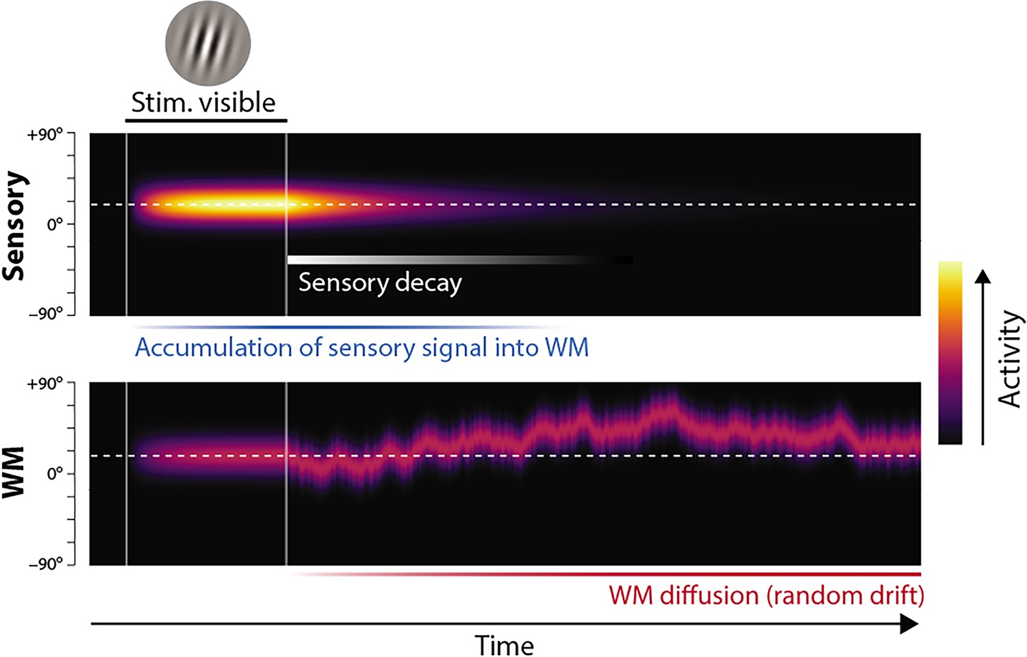
Proposed neural population dynamics for encoding a single orientation into visual working memory (VWM) and maintaining it over a delay.
Top: Stimulus onset is followed by a ramping increase in activity (indicated by color) of sensory neurons whose tuning (indicated on y axis) matches the stimulus orientation. Following stimulus offset, this sensory signal rapidly decays. The sensory signal, including its decaying post-stimulus component, provides input into VWM. Bottom: At stimulus onset, the VWM population begins to accumulate activity from the sensory population. This accumulation saturates at a maximum amplitude determined by global normalization. As the sensory activity decays, the activity in the VWM population is maintained at a constant amplitude, but accumulation of random errors causes the activity bump to diffuse along the feature dimension (y axis) over time, changing the orientation represented by the population. At recall, when the VWM population activity is decoded, accuracy of the recall estimate depends on both the orientation represented (center of the activity bump) and the fidelity with which it can be retrieved (determined by activity amplitude).
Figure 2
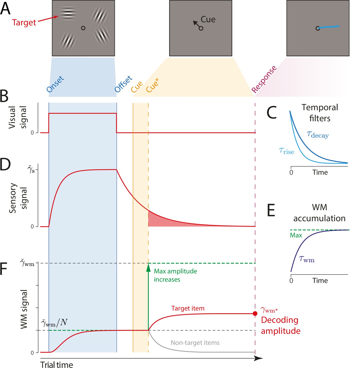
Schematic of signal amplitudes in the dynamic neural resource (DyNR) model during a cued recall trial.
(A) Observers are presented with a memory array (left), followed after a blank delay (not shown) by an arrow cue (center) indicating the location of one item (the target) whose remembered orientation should immediately be reported (right). (B) The amplitude of the visual input associated with each item is modeled as a step function (left). The sensory response (D) is modeled as a low-pass filtering of the stimulus input, with different time constants for rise and decay (C). (F) Amplitude of the working memory signal reflects a saturating accumulation of activity from the sensory population (illustrated in E). Beginning with stimulus onset, activity associated with each item is accumulated from the sensory population into the visual working memory (VWM) population, approaching an upper bound (green dashed line) that reflects a total activity limit shared between the items in memory. Once the cue has been presented (solid orange line) and processed (dashed orange line), uncued items can be dropped from VWM, raising the ceiling on activity available to represent the cued item (green arrow). This allows more information about the cued item to be accumulated from the decaying sensory trace (equivalent to the red shaded area in D). Response variability depends on the asymptotic VWM signal amplitude available for decoding (red circle) combined with the accumulated effects of diffusion (see text).
Figure 3
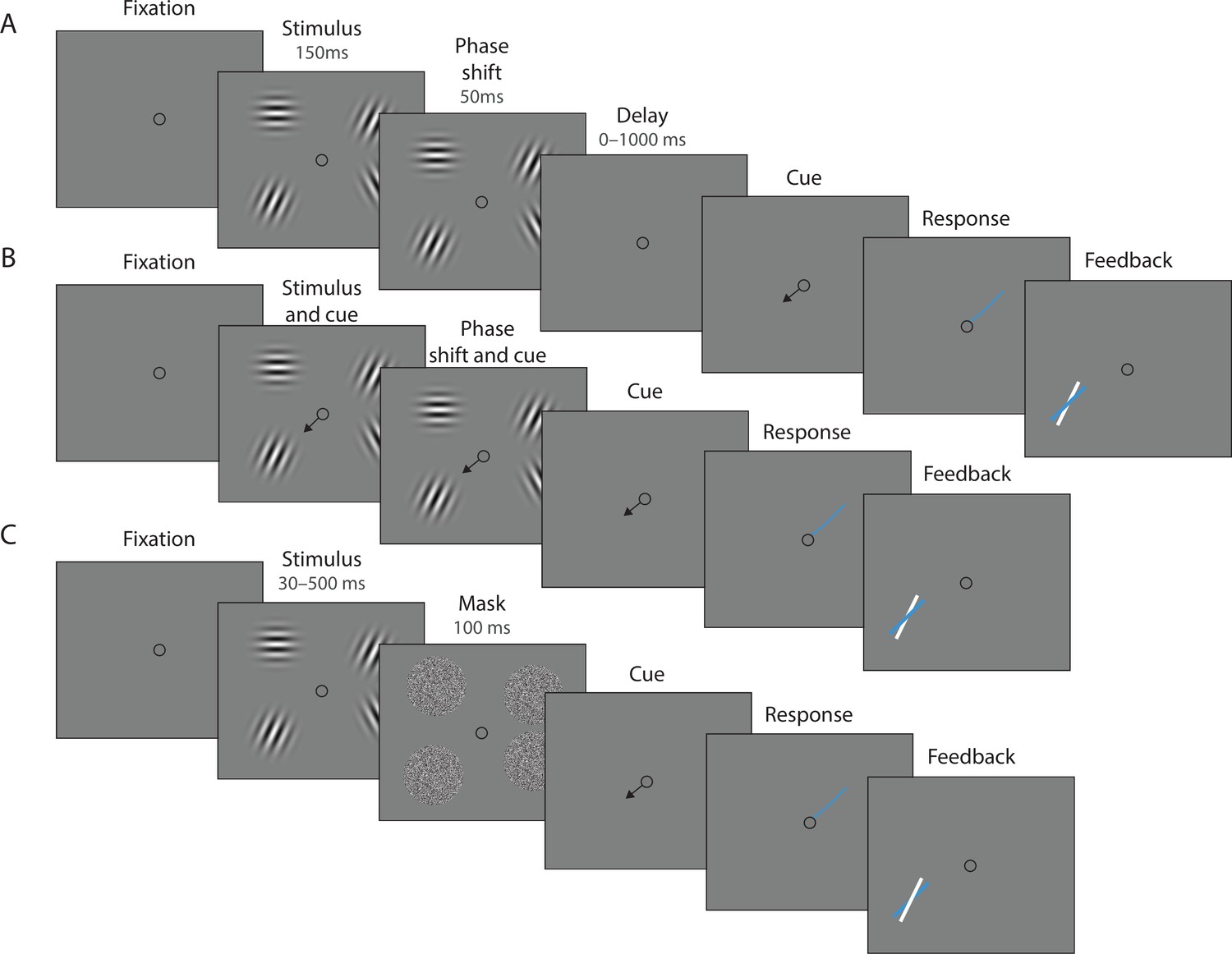
Experimental procedure.
(A) Experiment 1. On each trial, a memory array was presented consisting of 1, 4, or 10 randomly oriented Gabor stimuli. In 50% of all trials, the stimuli underwent a change of phase and contrast toward the end of the exposure period intended to minimize retinal after-effects. After a variable delay, an arrow cue was shown pointing toward the location of one stimulus from the preceding array. Observers reported the remembered orientation of the cued stimulus by swiping their index finger on the touchpad. The response was followed by feedback showing the true orientation. (B) In a proportion of trials, the cue was presented simultaneously with the stimuli. (C) Experiment 2. On each trial a memory array consisting of 1, 4, or 10 randomly oriented Gabor was presented for a variable duration, and followed by a white noise flickering mask. The mask was replaced by an arrow cue pointing toward the location of one stimulus from the preceding array. Observers reported remembered its orientation and received feedback as in Experiment 1. Stimuli are not drawn to scale.
Figure 4
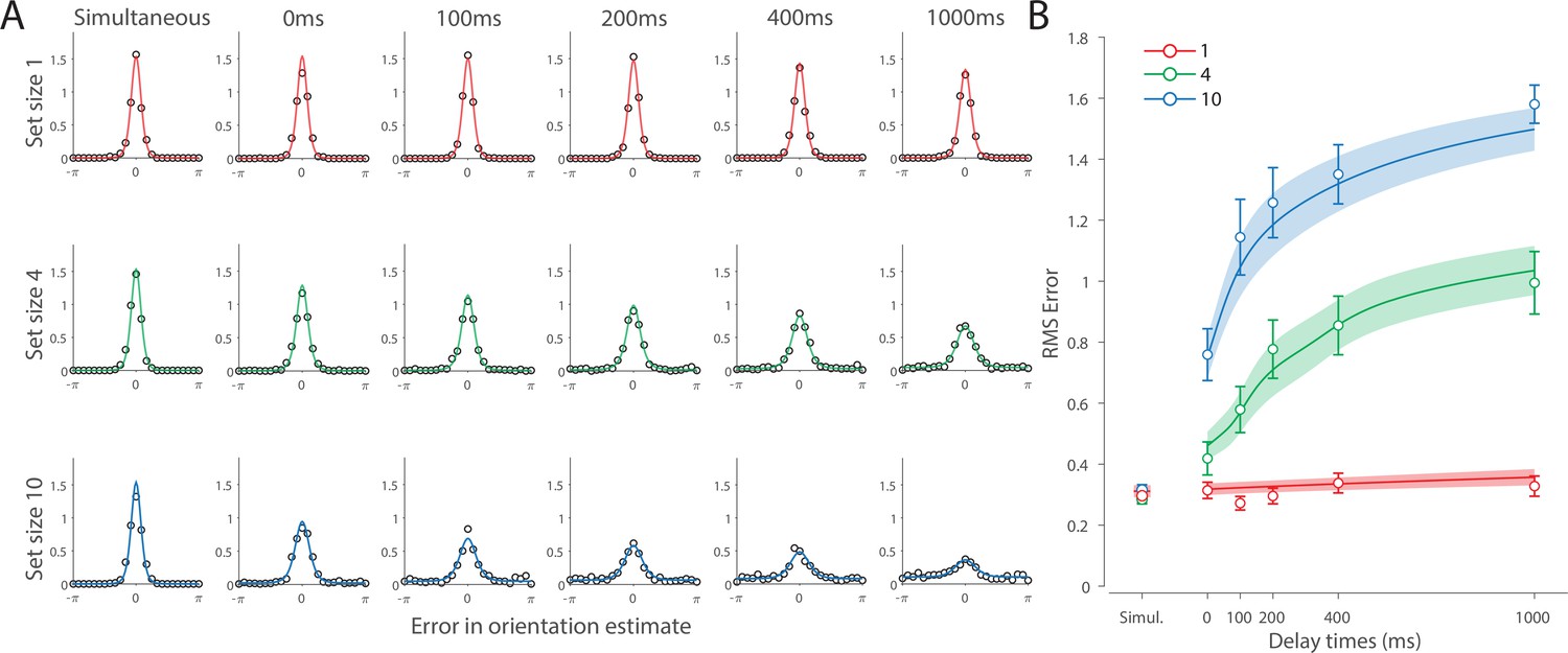
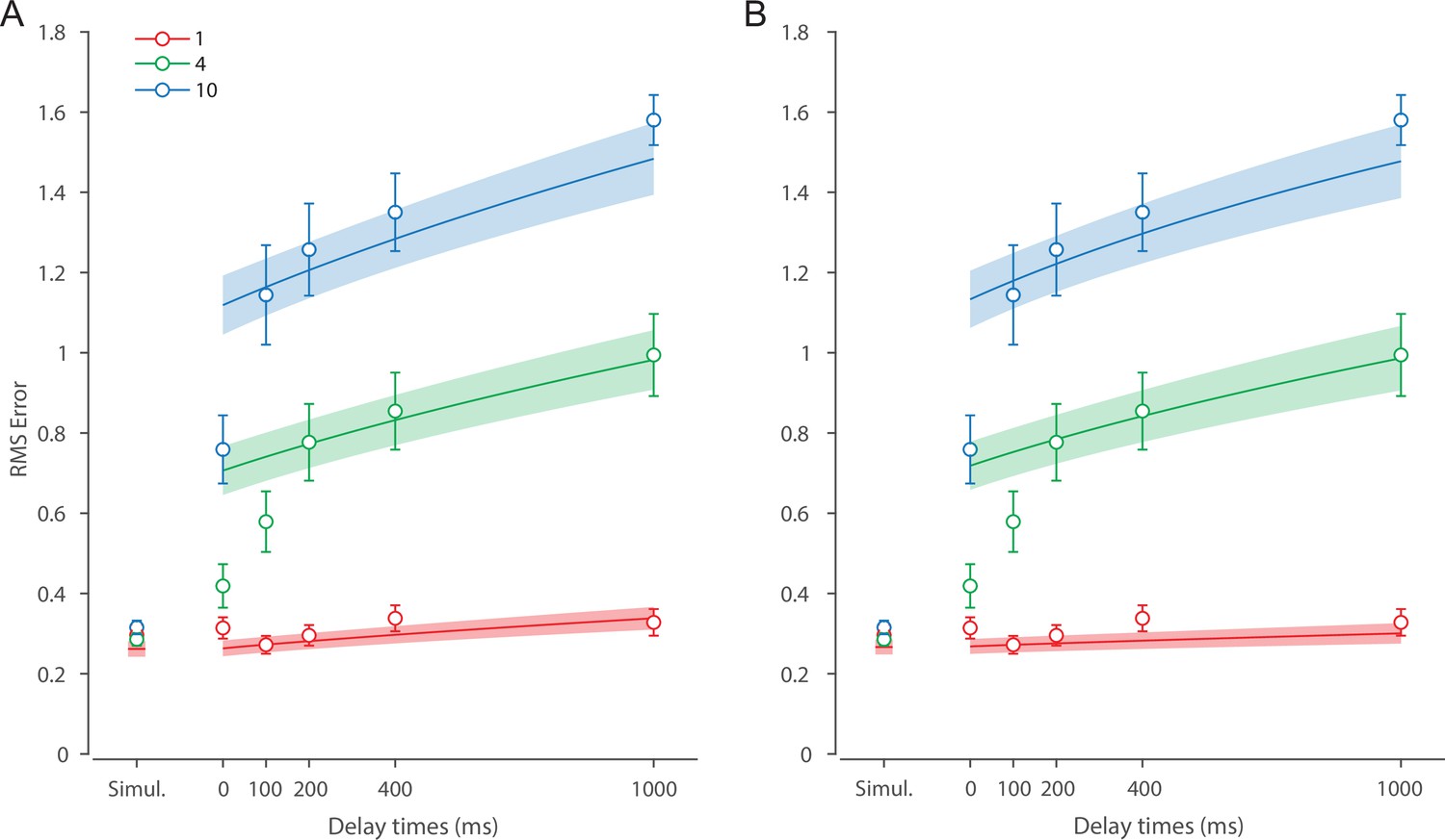
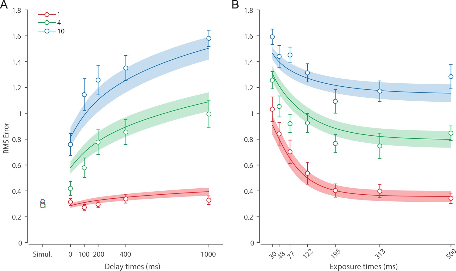
Experiment 1 data and model fits show the consequences of varying set size and delay duration on working memory (WM) reproduction error.
(A) Empirical recall error distributions (black circles) and the dynamic neural resource (DyNR) model fits (colored curves). Different panels correspond to different set sizes (rows) and delays (columns). (B) Corresponding RMS errors from experimental data (circles and error bars) and the DyNR model fits (curves and error patches). Error bars and patches indicate ±1 SEM. N = 10.
Figure 5
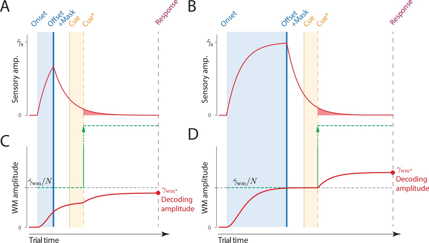
Time course of sensory and working memory (WM) gain with variable exposure duration.
(A, B) The signal amplitude in the sensory population increases from stimulus onset, exponentially approaching the maximum sensory activity (). For shorter presentation durations (A) the attained amplitude at stimulus offset is only a fraction of the maximum (compare B, late offset). Following offset, sensory areas produce a decaying neural response, that is curtailed (faster decay) but not abolished by a backward mask. (C, D) Information about the stimulus is accumulated in WM from sensory activity. A shorter presentation (C) provides less sensory evidence for the initial accumulation of all items into visual working memory (VWM) (compare D, late offset), and subsequently less decaying sensory activity that can supplement VWM activity for the target item following the cue.
Figure 6

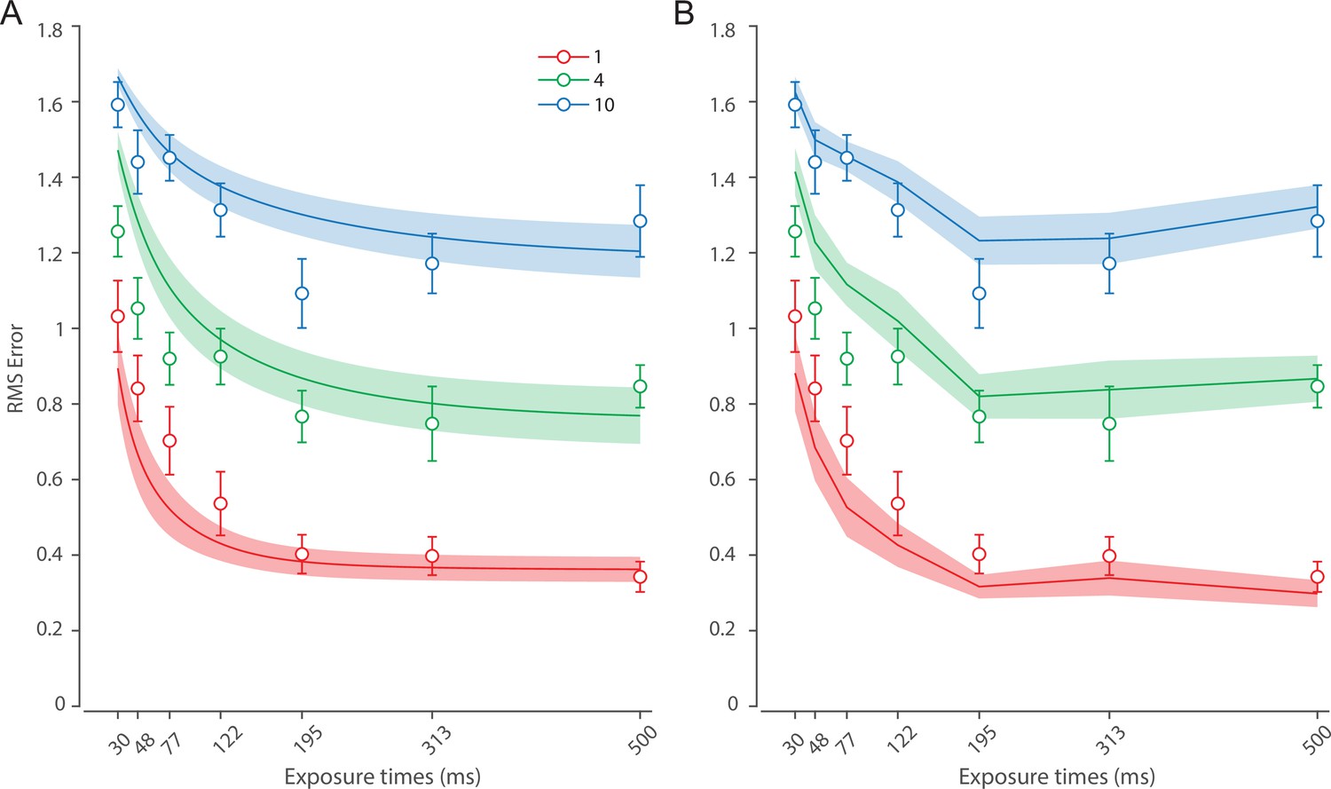
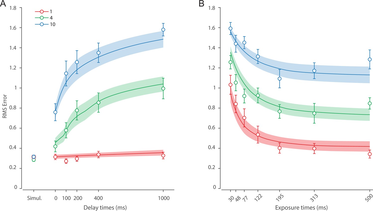
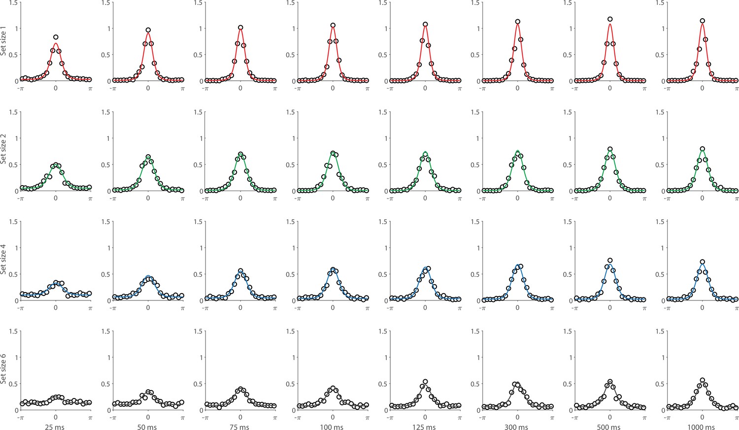
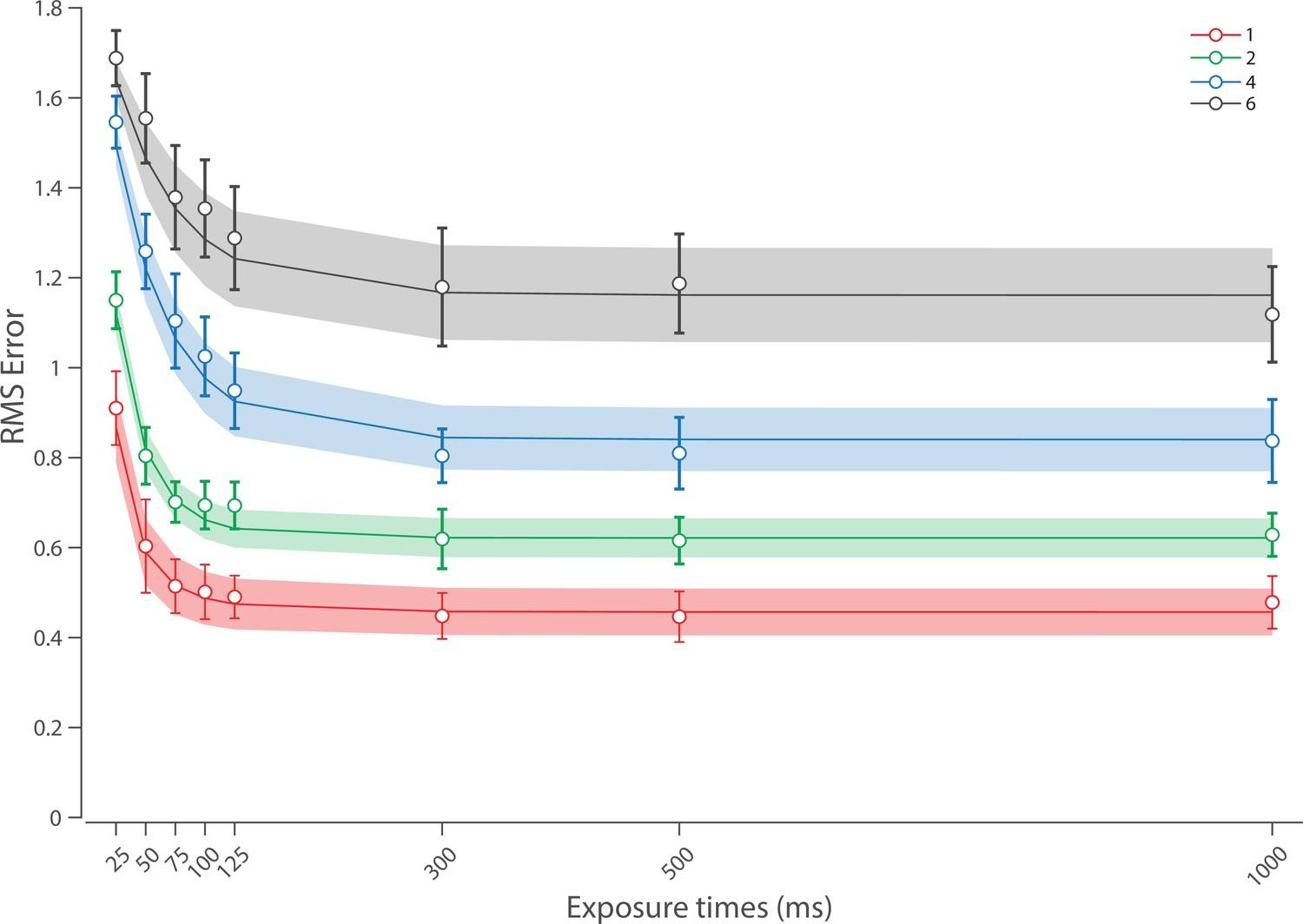
Experiment 2 results and modeling data show the consequences of varying set size and stimulus exposure time on visual working memory (VWM) reproduction error.
(A) Empirical recall error distributions (black circles) and the dynamic neural resource (DyNR) model fits (colored curves). Different panels correspond to different set sizes (rows) and exposure durations (columns). (B) Corresponding RMS errors from experimental data (circles and error bars) and the DyNR model fits (curves and error patches). Error bars and patches indicate ±1 SEM. N = 13.
Appendix 1—figure 1

Minimizing retinal after-effects.
Cancelling retinal afterimages. (A) Experiment 1 RMSE for trials without phase shift. (B) Differences in RMSE between trials with and without phase shift across set size and delay conditions. Negative values indicate better performance in the condition without phase shift. Error bars indicate ±1 SEM. N = 10.
Appendix 2—figure 1
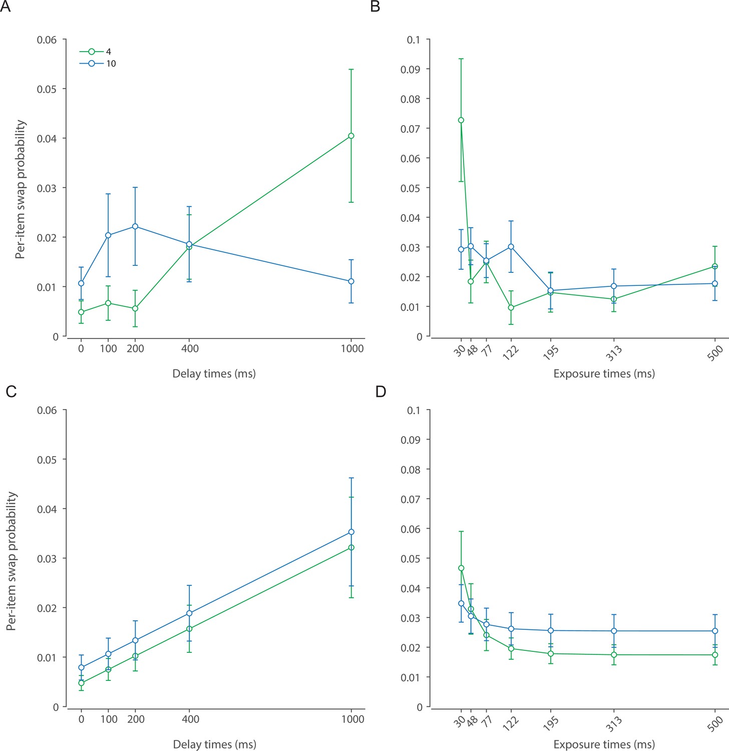
Swap error estimates.
(A and B) Probability of swap errors estimated from empirical data using the three-component mixture model (Bays et al., 2009) in Experiment 1 (A) and Experiment 2 (B). (C and D) Probability of swap errors in best-fitting dynamic neural resource (DyNR) model in Experiment 1 (N = 10) (C) and Experiment 2 (N = 13) (D). Error bars indicate ±1 SEM.
Appendix 3—figure 1
Experiment 1 behavioral data and model fit for the dynamic neural resource (DyNR) model without sensory persistence after stimulus offset.
(A) A version of the DyNR model with equal diffusion across set sizes. (B) A version of the DyNR model with diffusion that scales with set size. Error bars and patches indicate ±1 SEM. N = 10.
Appendix 3—figure 2
Experiment 2 behavioral data and model fit for the neural model without sensory persistence after stimulus offset.
(A) A version of the dynamic neural resource (DyNR) model without sensory persistence. (B) Separate fits of the simplified neural model to each exposure time. Error bars and patches indicate ±1 SEM. N = 13.
Appendix 3—figure 3
Behavioral data and model fit for a neural model with the direct read-out of information from sensory memory for (A) Experiment 1 (N = 10) and (B) Experiment 2 (N = 13).
Error bars and patches indicate ±1 SEM.
Appendix 3—figure 4
Behavioral data and model fit for the dynamic neural resource (DyNR) model without the cue processing time for (A) Experiment 1 (N = 10) and (B) Experiment 2 (N = 13).
Error bars and patches indicate ±1 SEM.
Appendix 3—figure 5
Behavioral data and model fit for a neural model with constant accumulation of information into working memory (WM) for (A) Experiment 1 (N = 10) and (B) Experiment 2 (N = 13).
Error bars and patches indicate ±1 SEM.
Appendix 4—figure 1

Experimental procedure.
Stimuli are not drawn to scale.
Appendix 4—figure 2
Behavioral data and model fit for Experiment 1a.
Error bars and patches indicate ±1 SEM. N = 10.
Appendix 5—figure 1
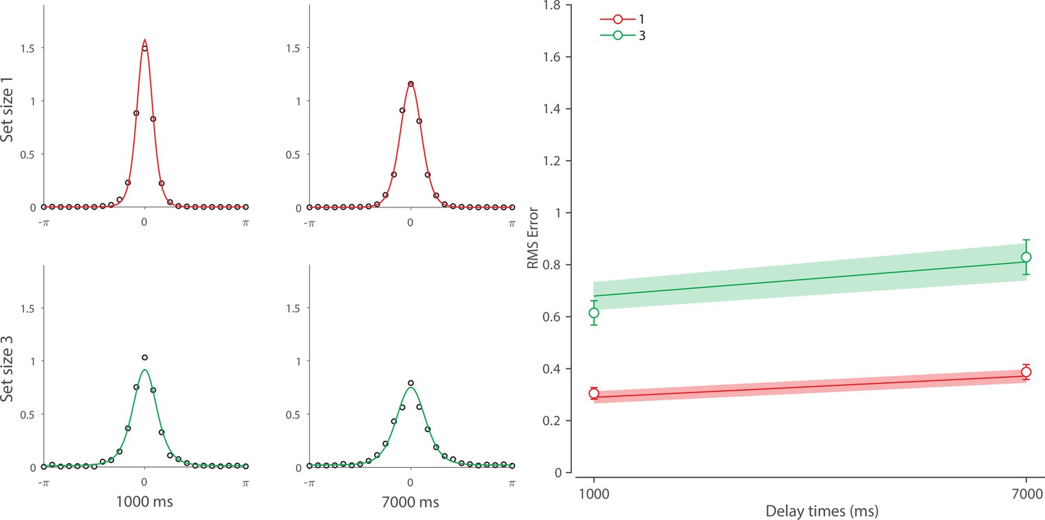
Empirical recall error distributions (black circles) from Experiment 1 in Bays et al., 2011, and the dynamic neural resource (DyNR) model fits to the data (colored curves).
Appendix 5—figure 2
Summary statistics (black circles) from Experiment 1 in Bays et al., 2011 and the dynamic neural resource (DyNR) model fits to the data (colored curves).
The DyNR model was fit to the distributions of recall errors shown in Appendix 5—figure 1. Error bars and patches indicate ±1 SEM. N = 32.
Tables
Table 1
Dynamic neural resource (DyNR) model parameters (1–9) and other variables (10–24) used in model description.
| No. | Parameter/variable | Description |
|---|---|---|
| 1 | Maximum VWM signal amplitude | |
| 2 | Tuning curve width | |
| 3 | Rise constant of the sensory temporal filter | |
| 4 | Decay constant of the sensory temporal filter | |
| 5 | Time constant of accumulation into VWM | |
| 6 | Base diffusion rate | |
| 7 | Time constant for spatial encoding | |
| 8 | Rate constant for spatial diffusion | |
| 9 | Scaling parameter for Hick’s law | |
| 10 | Time, relative to stimulus onset ( | |
| 11 | Time of stimulus offset | |
| 12 | Time of cue onset | |
| 13 | Time an item is identified for report | |
| 14 | Number of items in stimulus array | |
| 15 | Number of items in memory at time | |
| 16 | Maximum sensory signal amplitude | |
| 17 | Sensory signal amplitude at time | |
| 18 | VWM signal amplitude at time | |
| 19 | VWM signal amplitude at the time of decoding | |
| 20 | Accumulated diffusion at time | |
| 21 | Number of neurons | |
| 22 | True stimulus feature value | |
| 23 | Encoded stimulus feature value at the time of decoding | |
| 24 | Decoded stimulus feature value |
Additional files
Download links
A two-part list of links to download the article, or parts of the article, in various formats.
Downloads (link to download the article as PDF)
Open citations (links to open the citations from this article in various online reference manager services)
Cite this article (links to download the citations from this article in formats compatible with various reference manager tools)
A dynamic neural resource model bridges sensory and working memory
eLife 12:RP91034.
https://doi.org/10.7554/eLife.91034.3


