Figures and data in Distractor effects in decision making are related to the individual’s style of integrating choice attributes | eLife

Figures
Tables
Additional files

6 figures, 4 tables and 1 additional file

Figures

Figure 1

Download asset Open asset

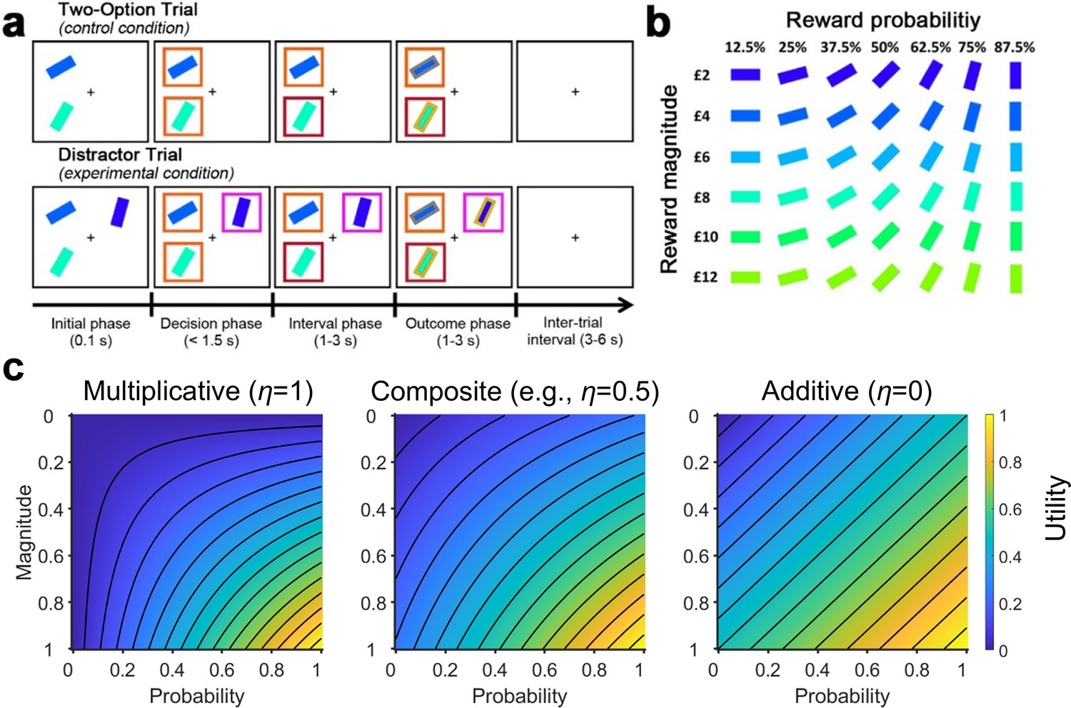
The multi-attribute decision making task (Chau et al., 2014; Gluth et al., 2018).

(a) On the control Two-Option Trials, participants were presented with two options associated with different levels of reward magnitude and probability, each in the form of a rectangular bar surrounded by an orange box. On the experimental Distractor Trials, three options were presented. Two options were subsequently surrounded by orange boxes indicating that they could be chosen, while a third option was surrounded by a purple box indicating that it was an unchooseable distractor. (b) The association between stimulus colour and orientation to reward magnitude and probability, respectively. Participants were instructed to learn these associations prior to task performance. (c) Plots illustrating utility estimated using (left) a purely multiplicative rule and (right) a purely additive rule (here assuming equal weights for probability and magnitude). By comparing their corresponding plots, differences in the utility contours are most apparent in the bottom-left and top-right corners. This is because in the multiplicative rule a small value in either the magnitude or probability produces a small overall utility (blue colours). In contrast, in the additive rule the two attributes are independent – a small value in one attribute and a large value in another attribute can produce a moderate overall utility (green colours). (Middle) Here, we included a composite model that combines both rules. The composite model involves an integration coefficient $η$ that controls the relative contributions of the multiplicative and additive rules.

© 2014, Springer Nature. Panels a and b are reproduced from Chau et al., 2014, by permission of Springer Nature (copyright, 2014). This figure is not covered by the CC-BY 4.0 licence and further reproduction of this panel would need permission from the copyright holder.

Figure 2

Download asset Open asset

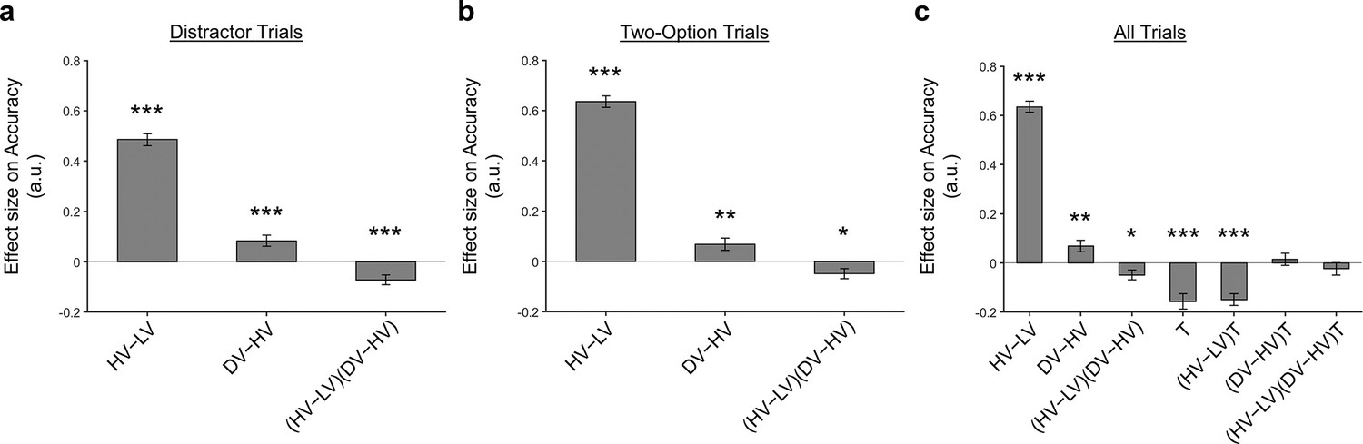
A distractor effect was absent, when the way participants combined choice attributes was ignored.

Although a positive distractor effect (indicated by the DV-HV term) was present on both (a) Distractor and (b) Two-Option Trials, (c) the distractor effects in the two trial types were not significantly different when they were compared in a single analysis [indicated by the $(D V - H V) T$ term]. Error bars indicate standard error. * p<0.05, ** p<0.01, *** p<0.001.

Figure 3 with 2 supplements

Download asset Open asset

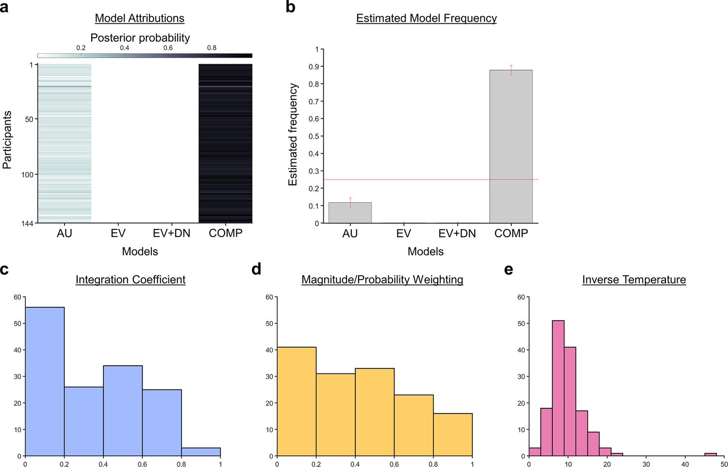
A Bayesian model comparison showed that the composite model provides the best account of participants’ choice behaviour.

(a) The posterior probability of each model in accounting for the behaviour of each participant. (b) A model comparison demonstrating that the composite model (COMP) is the best fit model, compared to the additive utility (AU), expected value (EV), and expected value and divisive normalisation (EV +DN) models. Histograms showing each participant’s fitted parameters using the composite model: (c) Values of the integration coefficient ( $0 \leq η \leq 1$ ), (d) magnitude/probability weighing ratio ( $0 \leq γ \leq 1$ ), and (e) inverse temperature ( $ϑ$ ).

Figure 3—figure supplement 1

Download asset Open asset

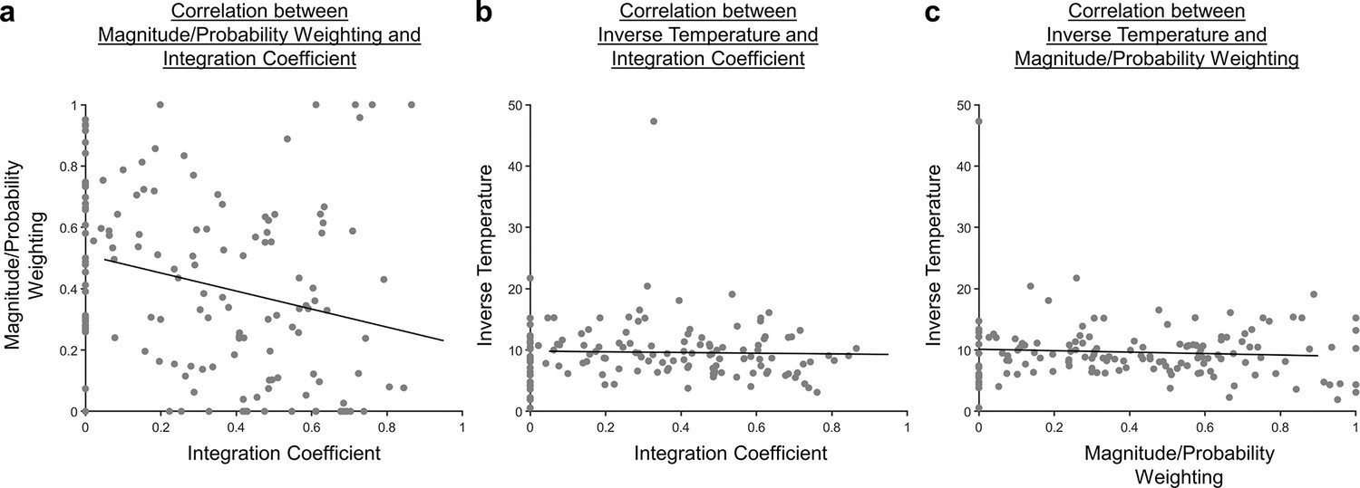
Scatterplots illustrating the correlation between the fitted parameters.

(a) The Pearson’s correlation between the magnitude/probability weighting and integration coefficient was significant [r(142)=−0.259, p=0.00170]. (b) The Pearson’s correlation between the inverse temperature and integration coefficient was not significant [r(142)=−0.0301, p=0.721]. (c) The Pearson’s correlation between the inverse temperature and magnitude/probability weighting was not significant [r(142)=−0.0715, p=0.394].

Figure 3—figure supplement 2

Download asset Open asset

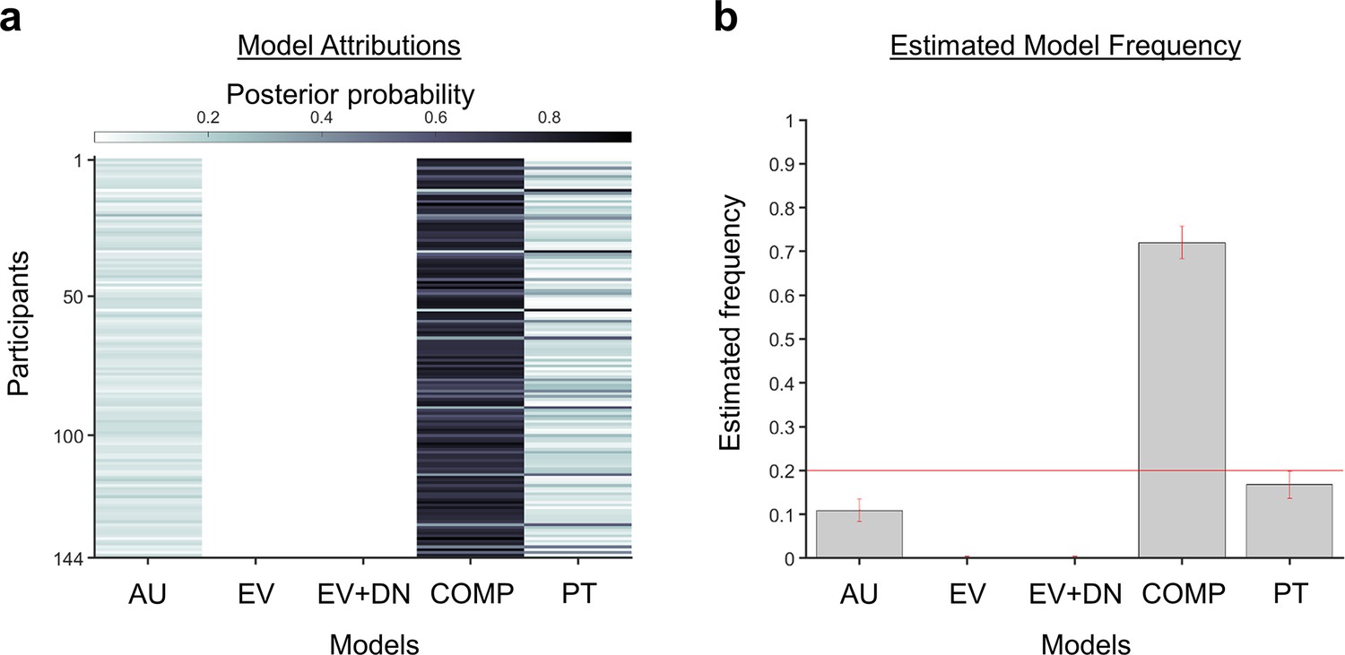
A Bayesian model comparison showed that the composite model provides the best account of participants’ choice behaviour even when a model with utility curvature based on Prospect Theory (Kahneman and Tversky, 1979) with the Prelec formula for probability (Prelec, 1998) is also considered.

${\bar{X}}_{i} = X_{i}^{α}$

${\bar{P}}_{i} = e^{- {(- \log P_{i})}^{β}}$

$P T_{i} = {\bar{X}}_{i} \times {\bar{P}}_{i}$

where 𝑋_𝑖 and 𝑃_𝑖 represent the reward magnitude and probability (both rescaled to the interval between 0 and 1), respectively. 𝑋̅𝑖 is the weighted magnitude and 𝑃̅𝑖 is the weighted probability, while 𝛼 and 𝛼 are the corresponding distortion parameters. (a) The posterior probability of each model in accounting for the behaviour of each participant’s behaviour. (b) A model comparison demonstrating that the composite model (COMP) is the best fit model (exceedance probability = 1.000, estimated model frequency = 0.720), compared to the additive utility (AU), expected value (EV), expected value and divisive normalisation (EV+DN), and prospect theory (PT) models.

Figure 4

Download asset Open asset

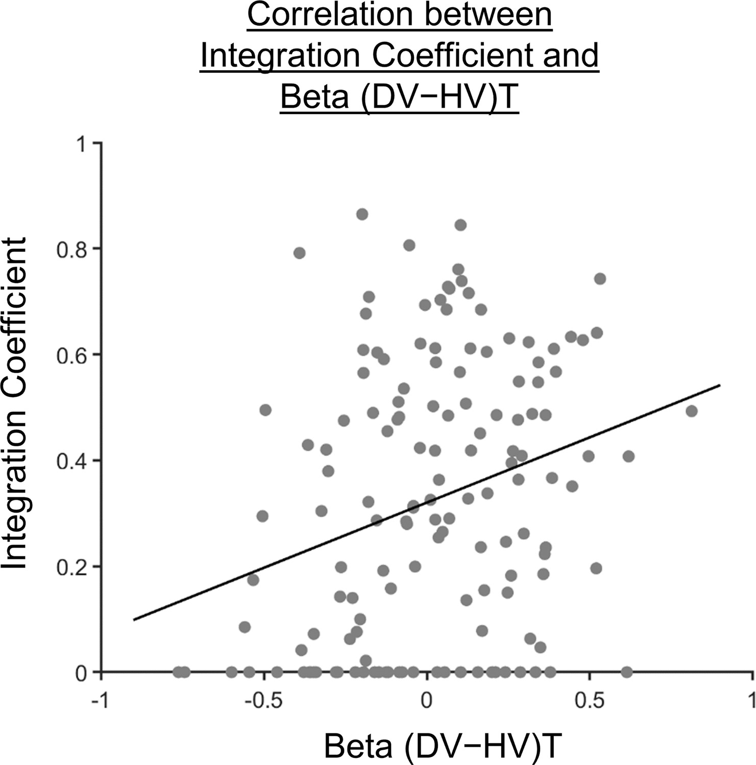
Participants showing a more multiplicative style of combining choice attributes into an overall value also showed a greater distractor effect.

A scatterplot illustrating a positive correlation between the integration coefficient ( $η$ ) and the distractor term (i.e. $(D V - H V) T$ ) obtained from GLM2 (Figure 2c). A significant positive correlation was observed [ $r (142) = 0.282$ , $p = 0.000631$ ].

Figure 5 with 3 supplements

Download asset Open asset

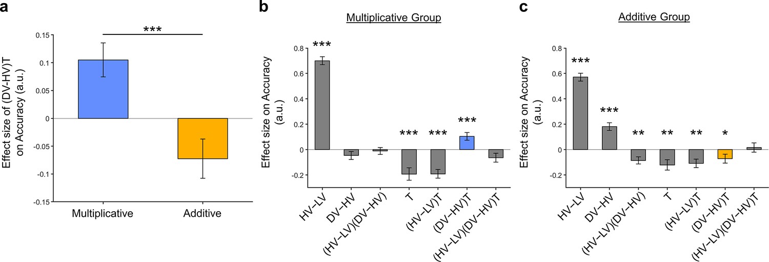
Significant distractor effects were found when participants’ styles of combining choice attributes were considered.

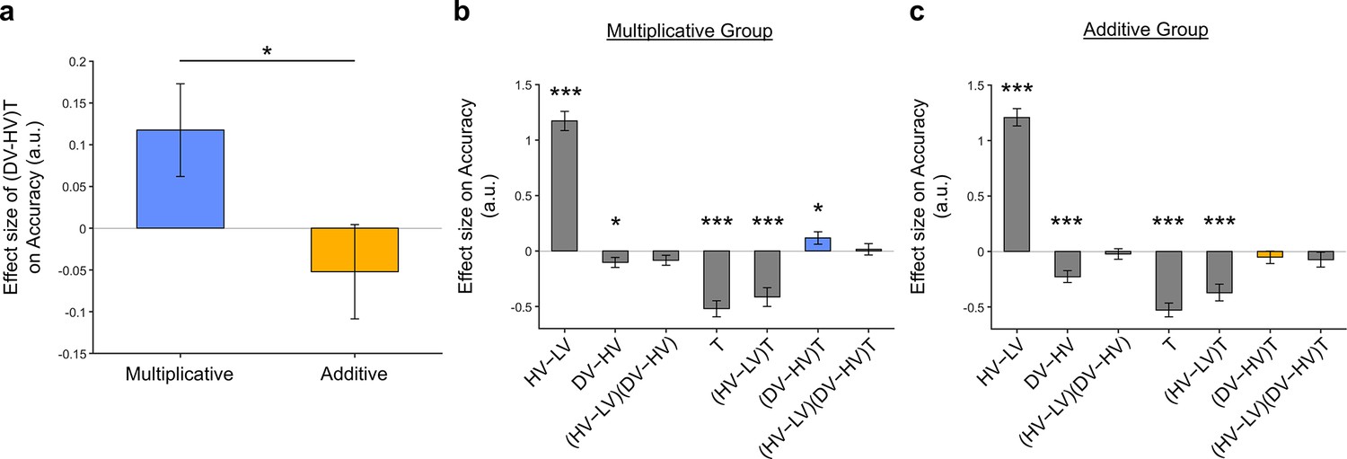
(a) A positive distractor effect, indicated by the $(D V - H V) T$ term, was found in the Multiplicative Group, whereas a negative distractor effect was found in the Additive Group. The $(D V - H V) T$ term was also significantly different between the two groups. Plots showing all regression weights of GLM2 when the data of the (b) Multiplicative Group and (c) Additive Group were analysed. The key $(D V - H V) T$ term extracted in (a) is highlighted in blue and yellow for the Multiplicative Group and Additive Group, respectively. Error bars indicate standard error. * p<0.05, ** p<0.01, *** p<0.001.

Figure 5—figure supplement 1

Download asset Open asset

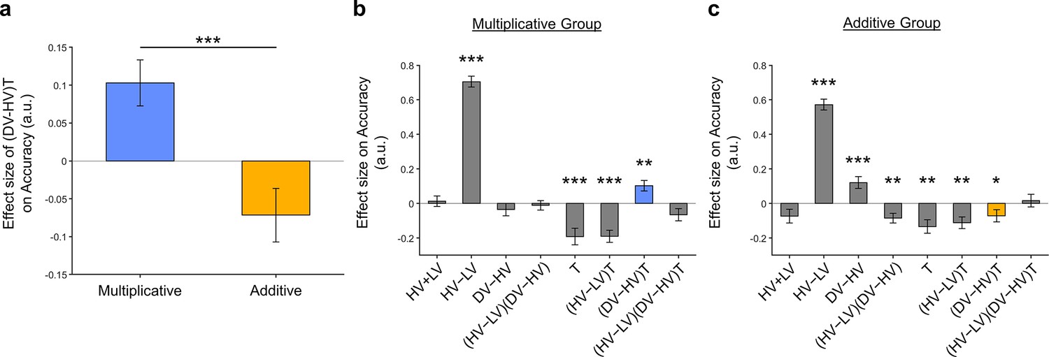
The distractor effects shown in Figure 5 remained significant after including an extra $H V + L V$ term in GLM3.

GLM3 differs from GLM2 only by including an extra $H V + L V$ term:

$\begin{array}{ll} L o g i t (a c c u r a c y) & = β_{0} + β_{1} z_{(H V + L V)} + β_{2} z_{(H V - L V)} + β_{3} z_{(D V - H V)} + β_{4} z_{(H V - L V)} z_{(D V - H V)} \\ + β_{5} T + β_{6} z_{(H V - L V)} T + β_{7} z_{(D V - H V)} T + β_{8} z_{(H V - L V)} z_{(D V - H V)} T + ε \end{array}$

Similar to Figure 5, here (a) we observe that a positive distractor effect (i.e. positive (𝐷𝑉 − 𝐻𝑉)𝑇 term) was significant in the Multiplicative Group and a negative distractor effect was significant in the Additive Group. The (𝐷𝑉 − 𝐻𝑉)𝑇 term was also significantly different between the two groups [𝑡(142) = 3.735, 𝑡 = 0.000271]. Plots showing all regression weights of GLM2 when the data of the (b) Multiplicative Group, and (c) Additive Group were analysed. The key (𝐷𝑉 − 𝐻𝑉)𝑇 term extracted in (a) is highlighted in blue and yellow for the Multiplicative Group and Additive Group, respectively. Error bars indicate standard error. * p < 0.05, ** p<0.01, *** p<0.001.

Figure 5—figure supplement 2

Download asset Open asset

The distractor effect between groups were maginally significant following the introduction of the $(H V + L V) T$ term to GLM3 and changing the $D V - H V$ terms to $D V$ to prevent collinearity between the regressors.

GLM4 is defined as:

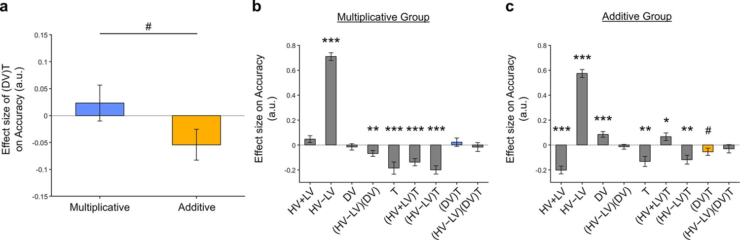
$L o g i t (a c c u r a c y) = β_{0} + β_{1} z_{(H V + L V)} + β_{2} z_{(H V - L V)} + β_{3} z_{(D V)} + β_{4} z_{(H V - L V)} z_{(D V)} + β_{5} T + β_{6} z_{(H V + L V)} T + β_{7} z_{(H V - L V)} T + β_{8} z_{(D V)} T + β_{9} z_{(H V - L V)} z_{(D V)} T + ε$

Despite not reaching significance, the distractor ‘effects’ in the Multiplicative Group and Additive Group maintained their positive and negative trends, respectively. (a) The distractor effects, indicated by the (𝐷𝑉)𝑇 term, were marginally significantly different between the two groups [𝑡(142) = 1.766, 𝑝 = 0.0796]. Plots showing all regression weights of GLM2 when the data of the (b) Multiplicative Group and (c) Additive Group were analysed. The key (𝐷𝑉)𝑇 term extracted in (a) is highlighted in blue and yellow for the Multiplicative Group and Additive Group, respectively. Error bars indicate standard error. # p < 0.08, * p < 0.05, ** p < 0.01, *** p < 0.001.

Figure 5—figure supplement 3

Download asset Open asset

The positive distractor effect in the Multiplicative Group shown in Figure 5 remained significant after replacing the utility function based on the normative Expected Value model with values obtained by using the composite model.

The distractor ‘effect’ in the Additive Group remained as a negative trend, despite not reaching significance. (a) A positive distractor effect, indicated by the $(D V - H V) T$ term, was found in the Multiplicative Group and the effects were also significantly different between the two groups [ $t (140) = 2.142$ , $p = 0.034$ ]. Plots showing all regression weights of GLM2 when the data of the (b) Multiplicative Group and (c) Additive Group were analysed. The key $(D V - H V) T$ term extracted in (a) is highlighted in blue and yellow for the Multiplicative Group and Additive Group, respectively. Error bars indicate standard error. * p<0.05, ** p<0.01, *** p<0.001.

Author response image 1

Download asset Open asset

Figure 4 after excluding 32 participants with integration coefficients smaller than 1×10-6.

Tables

Key resources table

Reagent type (species) or resource	Designation	Source or reference	Identifiers	Additional information
Software, algorithm	MATLAB R2022a	MATLAB	RRID:SCR_001622

Author response table 1

Regressor	beta_(1)	beta_(2)	beta_(3)	beta_(4)	beta_(5)	beta_(6)	beta_(7)
VIF	2.0799	2.0885	2.0089	1	2.0799	2.0885	2.0089

Author response table 2

Regressor	beta_(1)	beta_(2)	beta_(3)	beta_(4)	beta_(5)	beta_(6)	beta_(7)
VIF	2.0600	2.1433	2.1360	1	2.0600	2.1433	2.1360

Author response table 3

Regressor	beta_(1)	beta_(2)	beta_(3)	beta_(4)	beta_(5)	beta_(6)	beta_(7)	beta_(8)
VIF	2.5814	2.1014	3.7051	2.0136	1	2.0799	2.0885	2.0089

Additional files

MDAR checklist: https://cdn.elifesciences.org/articles/91102/elife-91102-mdarchecklist1-v1.docx
Download elife-91102-mdarchecklist1-v1.docx

Download links

A two-part list of links to download the article, or parts of the article, in various formats.

Downloads (link to download the article as PDF)

Open citations (links to open the citations from this article in various online reference manager services)

Mendeley

Cite this article (links to download the citations from this article in formats compatible with various reference manager tools)

Jing Jun Wong
Alessandro Bongioanni
Matthew FS Rushworth
Bolton KH Chau

(2024)

Distractor effects in decision making are related to the individual’s style of integrating choice attributes

eLife 12:RP91102.

https://doi.org/10.7554/eLife.91102.3

Sign up for email alerts

Privacy notice