Developing a crop- wild-reservoir pathogen system to understand pathogen evolution and emergence
- The Earlham Institute Norwich Research Park, United Kingdom
- National Institute of Agricultural Botany, United Kingdom
- IBM Research Europe, United Kingdom
- British Beet Research Organisation, United Kingdom
- Department of Life Science, The Natural History Museum, United Kingdom
Figures
Figure 1 with 1 supplement
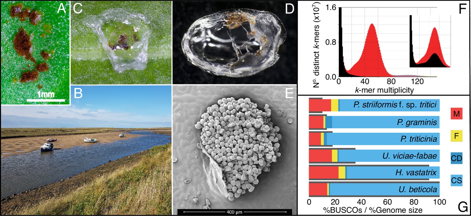
Zooming in on beet rust, pustules from wild and crop hosts are peeled and sequenced.
(A) U. beticola pustules on sugar beet. (B) Sea beets in their natural setting along an estuary, located bottom right and middle of the bank. Leaves are clipped and brought back into the lab. (C & D) Pustules are covered with 5 µl peel solution which dries and is peeled off for DNA extraction, library preparation, and sequencing. (E) An electron micrograph image of a rust pustule, isolate urediniospores are visible. (F) The rust genome k-mer spectra is a histogram of the number of k-mers (in the reads) found at a given multiplicity (or depth) at k-mers in the assembly. K-mers present in the reads but absent in the assembly are plotted in black, present once in the assembly in red, then purple for twice. The inset plot shows the k-mer distribution where all contigs without a blast hit are removed. The black peak within the main distribution indicates that real U. beticola content has been removed and should not be filtered from the assembly. (G) BUSCO completeness scores for our U. beticola (588.0 Mbp) genome in comparison to Hemileia vastatrix (541.2 Mbp), Uromyces viciae-fabae (209.5 Mbp), P. triticinia (106.6 Mbp), Puccinia graminis (81.5 Mbp) and P. striiformis f. sp. Tritici (61.4 Mbp). Colours indicate Missing, Fragmented, Complete and Duplicated, and Complete and Single copy BUSCOs. Genomes are in size order, represented as grey bars outlining BUSCO scores. The U. beticola genome, while large, has comparatively low levels of missing, fragmented, and duplicated BUSCO content.
Figure 1—figure supplement 1

Combined interspersed repeat content relative to genome size.
The U. beticola assembly contains a large proportion of interspersed repeat content (~90%). Analysis of repeat content across rust genomes (RepeatModeler RepeatMasker) shows a strong correlation between genome size and repeat content. Expansion of the U. beticola genome and proliferation of repeats is in line with the level observed in other rusts based on this significant positive correlation between genome size and repeat content in the rust genomes analysed.
Figure 2
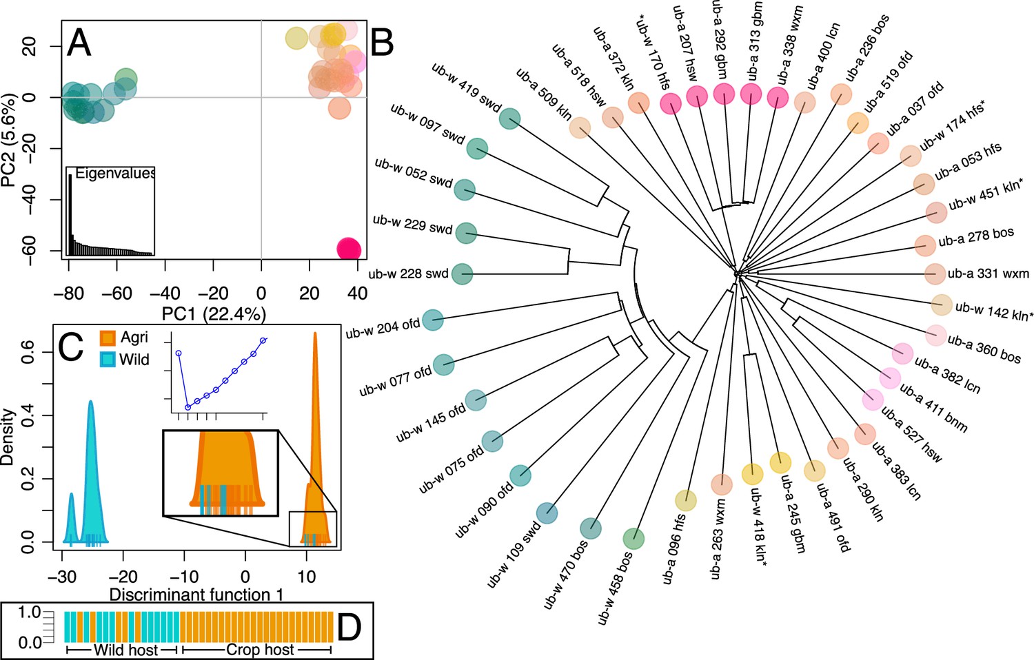
Population structure of wild and crop isolates.
(A) Principal Component Analysis of 300 thousand linkage-pruned SNPs. Principle Component 1 accounts for 22.4% of variance and divides isolates into two groups, the first (green-blue) contains only wild-infecting isolates, from southern sites. The second group (orange-pink), contains all crop-infecting isolates plus five northern wild sampled isolates. Five isolates are apart from the crop-infecting group on PC2 (5.6%). Only one of which is a wild-infecting isolate (ub-a_207_hsw ub-a_292_gbm ub-a_313_gbm ub-a_338_wxm ub-w_170_hfs). Isolates are coloured according to their position on each axis. Eigenvalues are represented, inset bottom left. (B) Neighbour Joining tree (coloured according to PCA) reflects the relationship in the PCA and shows that northern wild isolates (asterisks) are not more closely related to each other than they are to other crop-infecting isolates. (C) Discriminant analysis of principal components (DAPC) of 1.87 million SNPs. Bayesian information criterion (BIC) shows that (k=2) two clusters best describe the data (inset top: x=No. clusters, y=BIC) and so isolates are plotted over a single discriminant function (DF1). Isolate ticks are coloured by host sampling group (wild = cyan, crop = orange) and distributions are coloured by predominant membership to indicate a population containing only wild isolates and a population containing all agricultural isolates along with 5 northern wild isolates. Groups are coherent between PCA and DAPC analyses as well as being entirely disentangled on the DAPC plot. (D) The probability of the strain belonging to each group is equal to 1, ordered by host type and coloured by population (agri = orange, wild = cyan).
Figure 3
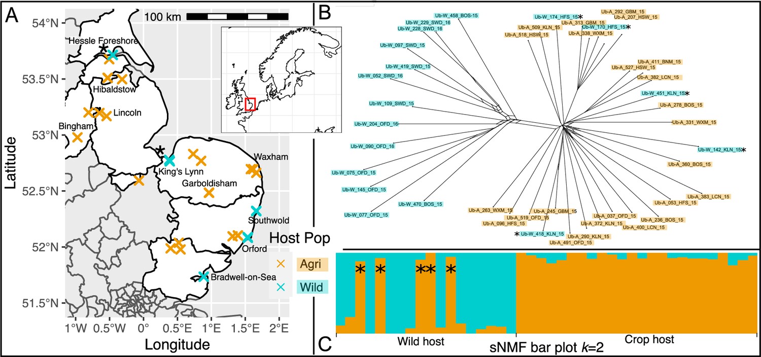
Spatial population structure and introgression of wild and crop isolates.
(A) Map of part of the UK shows samples coloured by host (crop = cyan, and wild = orange). Overlapping crosses obscure wild samples which can be distinguished using Supplementary file 2. Northern wild samples are accompanied by an asterisk (continued throughout the figure) because they are found within the crop clade (see B & C, and Figure 2). (B) SplitsTree network generated using the gene coding sequence (CDS) regions present in all isolates (15.2 Mbp) shows a clear differentiation of an exclusively wild population from all crop isolates plus five wild isolates. Population clustering and admixture analysis (sparse non-negative matrix factorization, sNMF; C) shows two partitioned populations in which the five northern isolates sampled on wild host belong to the crop cluster, with no increased signal of hybridisation.
Figure 4
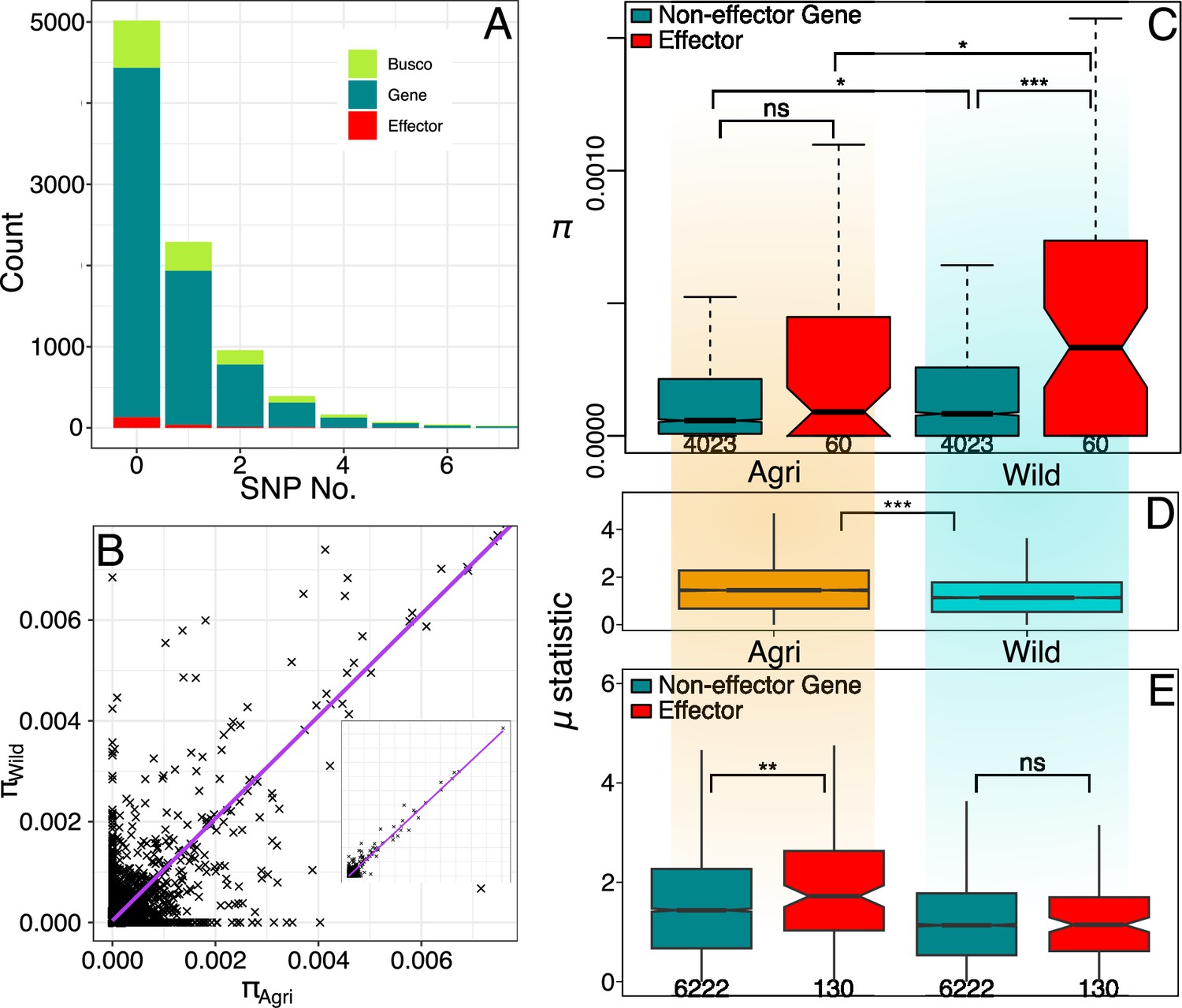
Wild effector genes maintain diversity.
(A) Histogram of gene numbers with a given number of SNPs in the coding sequence (CDS) region (0–7 SNPs). This diversity is measured from both populations combined and shows that polymorphism is low, over half of genes don’t contain a SNP within their coding region. (B) Nucleotide diversity present in gene CDS regions is strongly correlated between wild and crop populations. The inset shows the full range (0.00–0.05). (C) Nucleotide diversity present in polymorphic effector and non-effector gene CDS regions (shaded by population: Agri = orange, Wild = cyan). Agricultural non-effector genes have significantly less diversity than wild non-effector genes. Maintenance of polymorphism in wild effectors, is significantly greater than wild non-effectors and the maintenance of effector polymorphism is greater in the wild than in agriculture. The distinction between effector and non-effector genes is not significant in the agricultural population where diversity is more limited. (D) Raised accuracy in sweep detection (RAiSD) selective sweep μ statistic (50 kbp windows) plotted for all contigs (>50 kbp) from each population. The μ statistic is significantly greater on average in the agricultural population and the μ statistic plotted across each effector and non-effector gene (E) shows that agricultural effectors have significantly higher μ statistic values than non-effector genes. There is no similar significant difference in the wild population. Numbers of polymorphic genes and windows are presented under boxplots see (Source data 1).
Figure 5
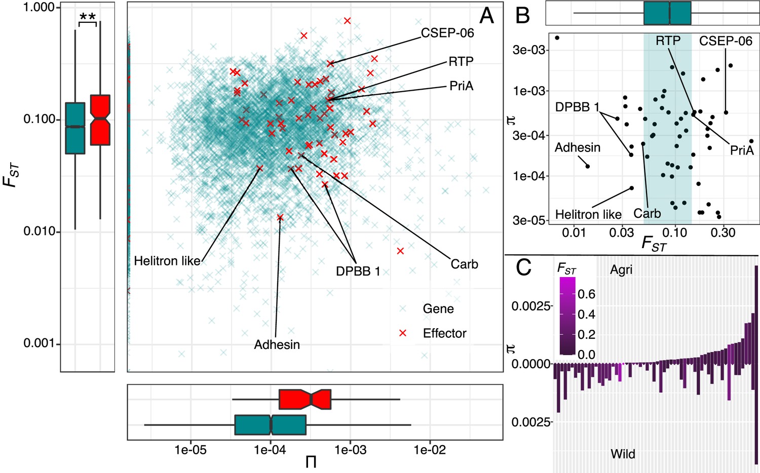
Evidence for adaptation is present in effector diversity.
(A) Levels of nucleotide diversity plotted against genetic differentiation of effector (red) and non-effector genes (green). Genetic differentiation is significantly greater in effectors than non-effectors which suggests that more genes in this group are exposed to diversifying selection, favouring variation specific to each environment. (B) Polymorphic effectors are plotted against the non-effector FST distribution, highlighting those effectors in the upper and lower ranges. (C) Polymorphic effectors plotted in order of agricultural nucleotide diversity underlines the importance of assessing agricultural diversity against a non-crop background, because this highlights those effectors, that are fixed in agriculture, are those that are most differentiated. Known effector functions in the upper and lower ranges are included (A & B, see Source data 1).
Figure 6
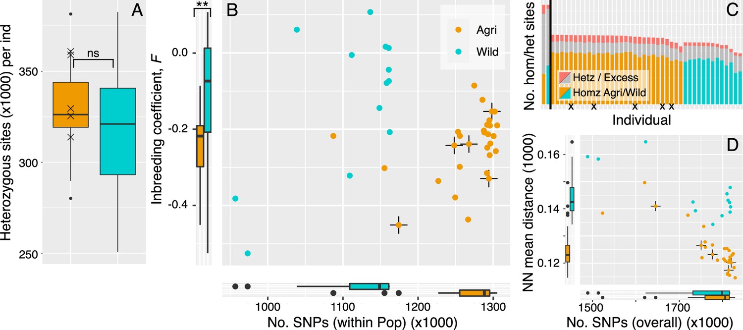
Clonality may be prioritised in the crop lineages.
(A) The level of heterozygosity is not significantly different between crop and wild populations. Isolates that cluster within the crop population but were isolated on a wild host, are marked by cross in each panel. (B) Numbers of SNPs per isolate (within population), plotted against inbreeding coefficient (FIS). Wild rust isolates have fewer SNPs segregating within population and broadly distributed FIS values that tend more towards zero and above. Crop isolates have larger numbers of SNPs (within population) and FIS values that are significantly more negative on average. Negative FIS values are indicative of a heterozygous excess and consistent with clonal modes of reproduction, as are accumulation of mutations at the isolate level. (C) Numbers of homozygous and heterozygous SNPs per isolate (across all isolates). Each isolate is represented by a single bar where homozygous sites coloured by population (Agri = orange, Wild = cyan). Grey with red tips represents the number of heterozygous sites per isolate with the red tips indicating the proportion of those heterozygous sites that are in regions of excess heterozygosity. The vertical black line separates population total values (left, reaching 1.87 million SNPs) from isolate values (right). (D) Numbers of SNPs per isolate, here SNPs are in relation to all other isolates plotted against mean pairwise Neighbour-Net distance among all isolates, compared to panel B.
Appendix 2—figure 1
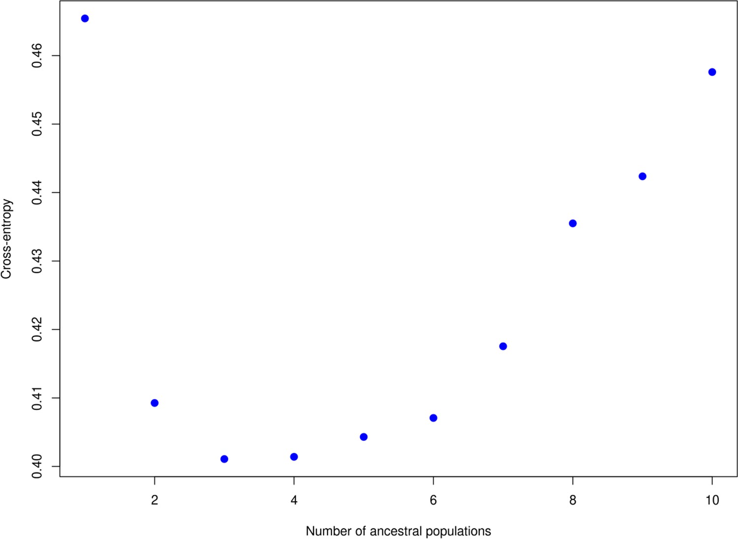
The ‘knee’ in the entropy criterion.
Used to define the number of clusters, which here is at two or three. A similar plot produced using DAPC is available in Figure 2 of the main text which indicates two populations.
Appendix 2—figure 2
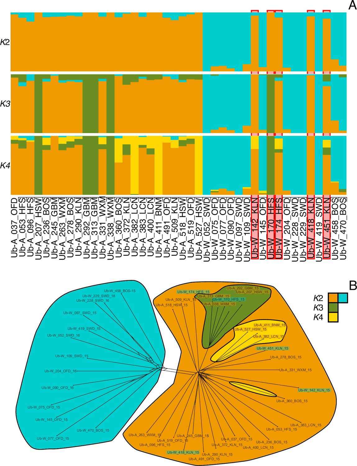
Bar plots of individual admixture of rust isolates.
(A) Admixture proportions for each individual for K=2:4. Isolates are ordered in two blocks as being sampled from a crop (Ub-A…) or a wild host (Ub-W…). The five wild sampled individuals that were identified to be within the crop infecting populations are bordered in red. (B) Network of relatedness (Figure 3B main text) among isolates. Sample name highlighting reflects host affiliation (crop = orange, wild = turquoise). Clade colouring reflects individual majority assignment colour from A.
Appendix 2—figure 3
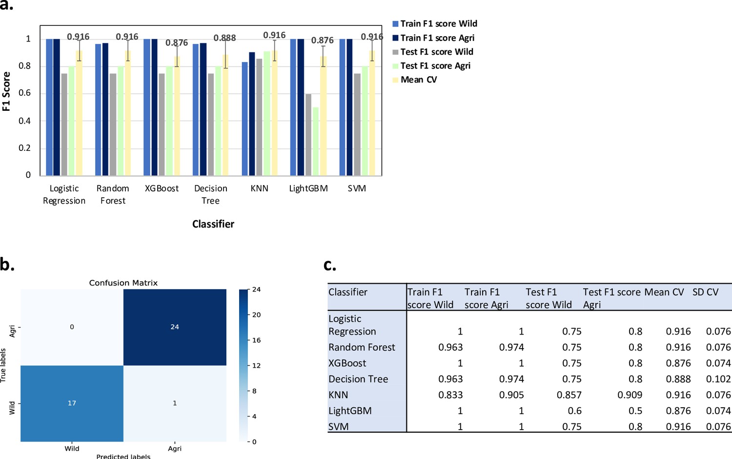
Results from ML classification analysis using 813,649 SNPs.
For the ML analysis to predict Wild/Agricultural in binary classification: (a) Bar charts showing the F1 scores for the training and test datasets (using best parameters) and the mean F1 scores (Mean CV) after fivefold cross validation with the standard deviation shown as error bars. Labels for different bar colours are detailed in legend to the right of the plot. (b) Confusion matrix for the KNN ML model for the training + test dataset i.e., all samples. (c) Table of performance values for each ML model as shown in (a).
Appendix 2—figure 4
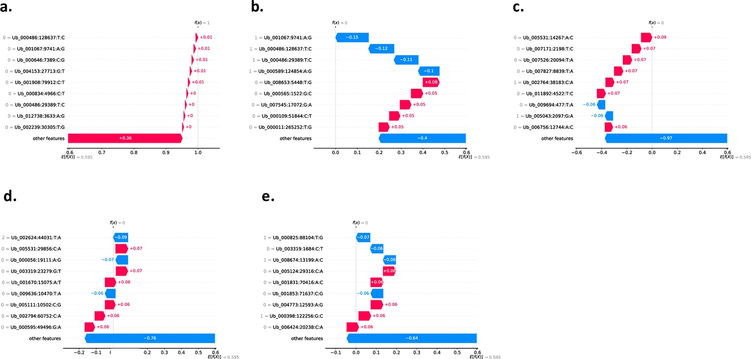
Using SHAP to explain our KNN binary classification model using 813,649 SNPs.
Here, we show the local explanation for the prediction of the five wild sampled individuals (a) Ub-w_142_kln that the model predicted as class 1=Agri. (b) Ub-w_170_hfs that the model predicted as class 0=Wild. (c) Ub-w_174_hfs that the model predicted as class 0=Wild. (d) Ub-w_418_kln that the model predicted as class 0=Wild. (e) Ub-w_451_kln that the model predicted as class 0=Wild. All plots (a–e) show the top 10 most impactful SNP alleles and their respective impact scores (most impactful ordered from top to bottom) that contributed to the classification of each sample as class 1 (Agri) as calculated using SHAP. The red colours denote an impact score for a SNP allele that has positively impacted the classification of the sample i.e., if we sum all SNP allele impact scores for a sample, a more positive score tending towards 1 gives the sample a classification of class 1 (Agri). The blue colours denote an impact score for a SNP allele that has negatively impacted the classification of the sample i.e., if we sum all SNP allele impact scores for a sample, a more negative score tending towards 0 gives the sample a classification of class 0 (Wild). Sample (a) Ub-w_142_kln was called class 1 (Agri) by the model and samples (b–e) Ub-w_170_hfs, Ub-w_174_hfs, Ub-w_418_kln, Ub-w_451_kln were called class 0 (Wild) by the model. In grey next to each SNP denotes the specific allele that the sample has i.e., Reference Homozygous SNPs (0/0) denoted as 0, Heterozygous SNPs (0/1) as 1, Homozygous SNPs (1/1) denoted as 2.
Appendix 3—figure 1
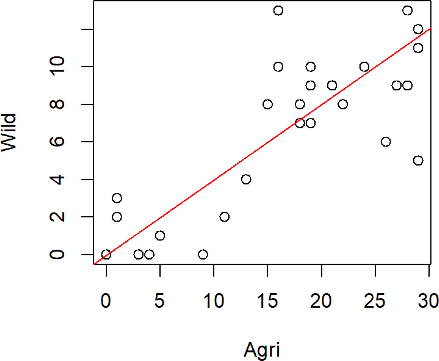
Missingness of genes from both the wild and agricultural populations (populations defined using DAPC).
For all non-effector genes that are missing in any one isolate, we present the number of isolates containing that gene in each population (r2=0.89 p=<2.2e-16). Most genes (48) are absent both populations.
Appendix 3—figure 2

Histogram of counts of observed effector and non-effector gene coding sequence (CDS) lengths (between 1-3500 bp) shows counts per gene type.
Vertical black lines indicate the effector length range.
Appendix 4—figure 1
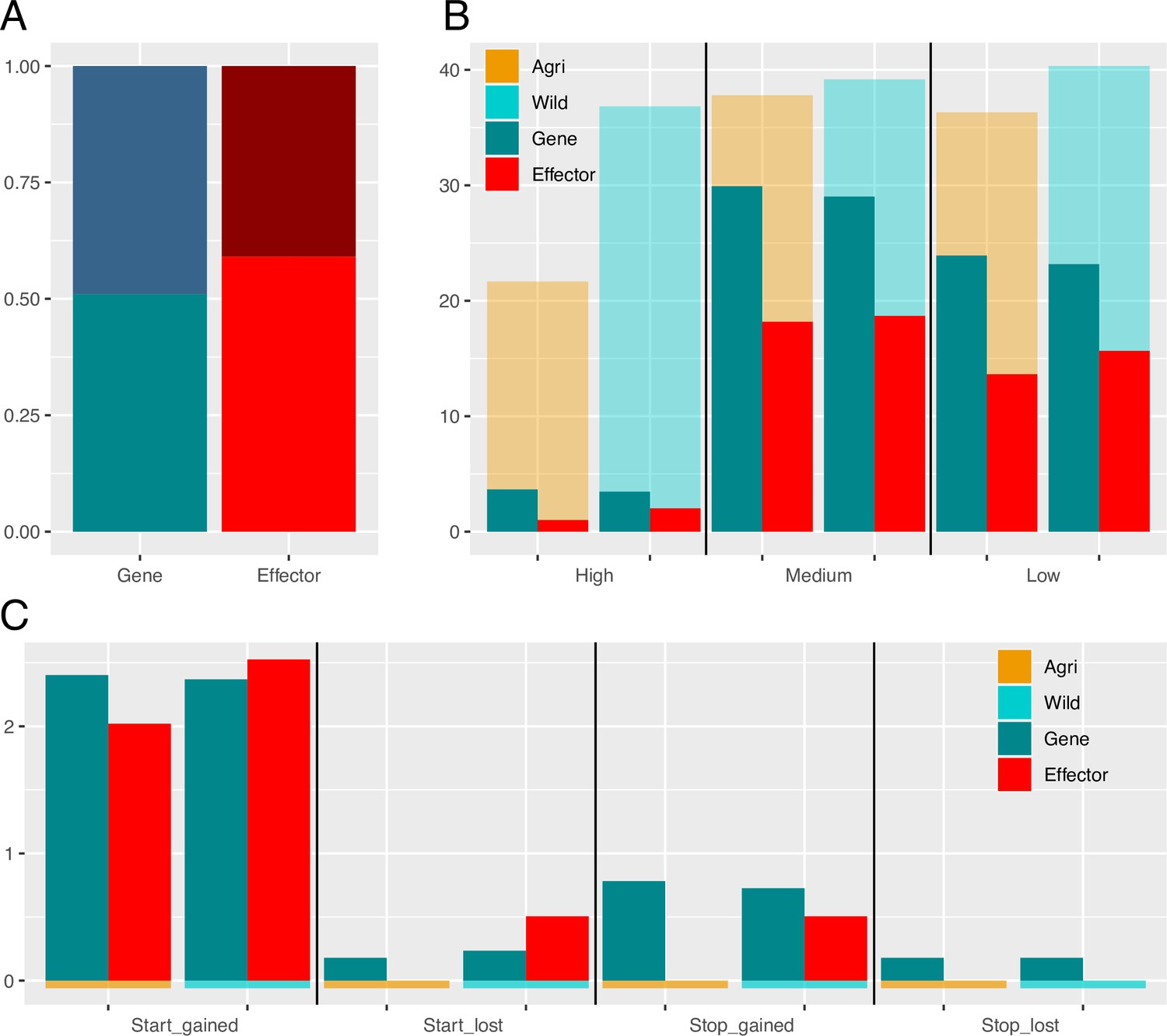
Alternative splicing and variant impacts in non-effector genes and effectors.
(A) Proportions of alternatively spliced genes is greater than that of effectors (shaded region is alternatively spliced). (B) Percentages of Genes (turquoise) and Effectors (red) with High, Medium, and Low impact variants (SNPs and indels combined). As expected based on average gene length there are a greater percentage of non-effector genes with variants (in all classes). Orange and blue backed bars reflect the percentage of mutated effectors relative to genes in each population. While a greater percentage of genes carry a polymorphism, the relative proportion of effectors that carry a polymorphism is always higher in the wild, compared to agricultural. (C) Percentages of genes and effectors impacted by start and stop, gained and lost polymorphisms.
Appendix 4—figure 2
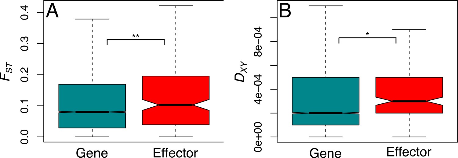
Genetic differentiation and divergence are significantly greater at effector loci.
Genetic differentiation (FST, A) and genetic divergence (DXY, B) present at effector and non-effector genes, reanalysed using 10 kb windows across all-sites. Genetic diversity and differentiation, are both significantly greater in effectors than non-effectors (see main text) which suggests that more genes in this group are exposed to diversifying selection, favouring effector polymorphism specific to each environment.
Appendix 4—figure 3
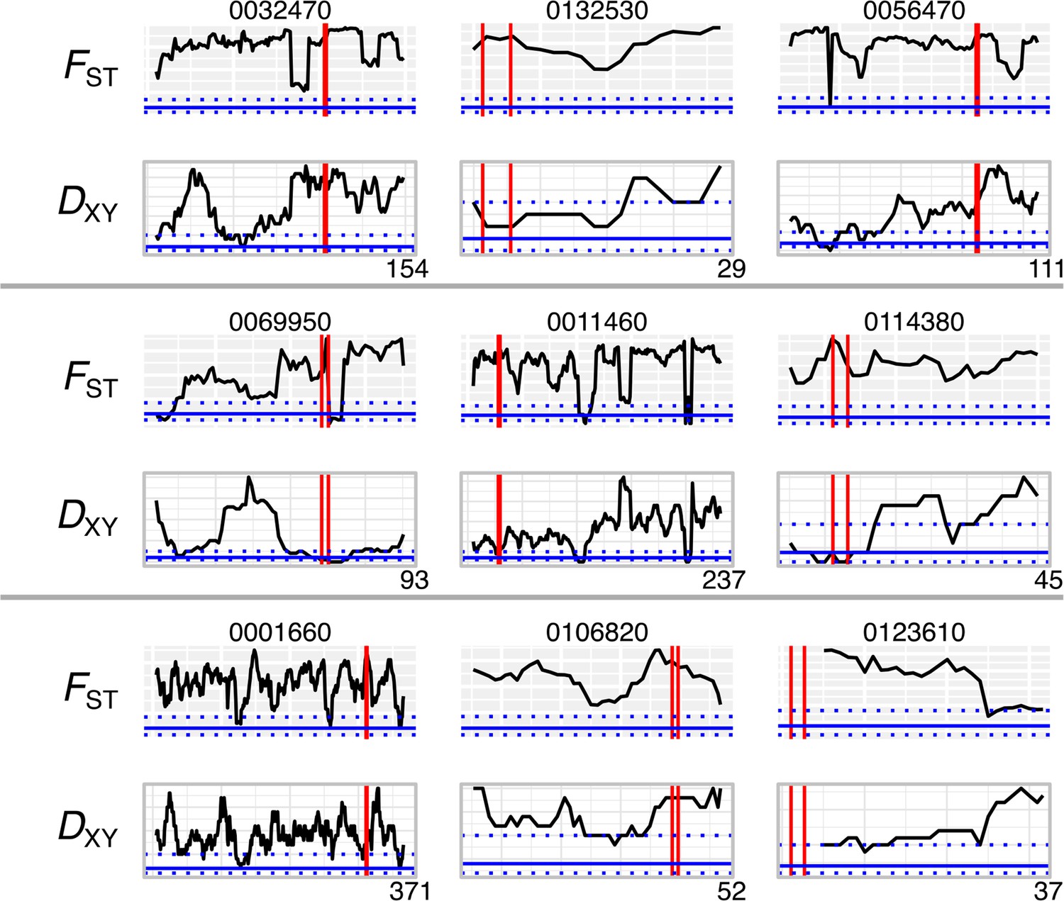
Genetic differentiation (FST) and divergence (DXY) for most differentiated effectors.
Windows of 10 kb across contigs containing effectors with the highest FST values, shown above (shaded background) and DXY below (clear background). Vertical red lines show the start and end position of the effector, and horizontal blue lines show the median and interquartile range for all genes. Contig lengths shown on x-axis (kb).
Appendix 5—figure 1
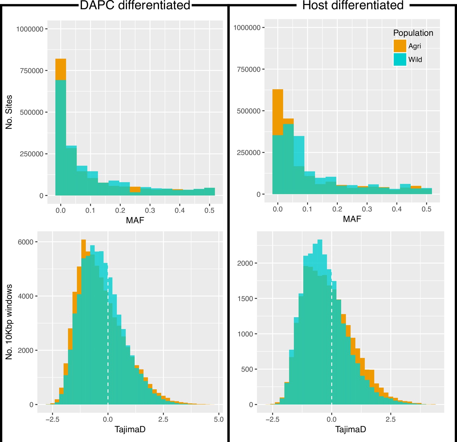
Minor allele frequency (MAF, top) and Tajima’s D (bottom) for all variants.
MAF and Tajima’s D analysed twice, once for each of the two methods of grouping these individuals (DAPC, left and Host differentiated, right; see Source data 1).
Appendix 5—figure 2
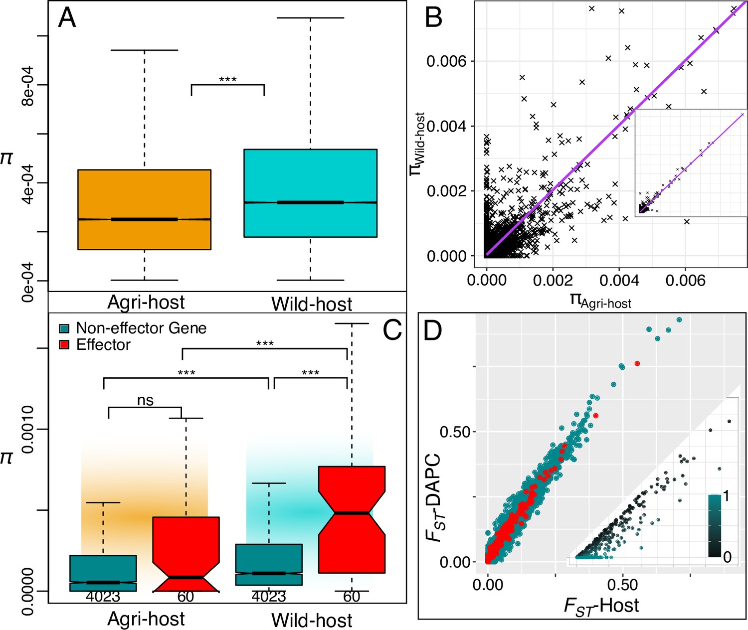
Host defined groups retain a signal of adaptive diversity in effectors.
(A) Genome wide nucleotide diversity (π, 10 kbp non-overlapping blocks) is significantly higher in the wild host-group compared to the agricultural-host group and (B) at the gene level, nucleotide diversity within the gene coding sequence (CDS) is strongly correlated between agricultural-host and wild-host groups. The inset shows the full range (0.00-0.05). (C) Comparing nucleotide diversity at effector (red) and non-effector genes (turquoise) we observe again that wild-host effector diversity is higher than both wild-host non-effector gene diversity and agricultural effector diversity. Gene CDS regions polymorphic in one or other population are plotted (see gene n under boxplot). (D) Genetic differentiation (FST) plotted for gene regions (5 kb up- and down-stream) for both host-differentiated, and population-differentiated groups. The there is a strong positive correlation in genetic differentiation between both grouping methods (Host and DAPC). Host differentiated groups are lower on average. The inlayed plot displays all 272 non-effector genes that have a higher genetic differentiation for Host-differentiated groups than DAPC-differentiated, the relative difference is displayed in the colour gradient. There were zero effector genes that had higher differentiation in Host relative to DAPC groupings (see Source data 1).
Tables
Table 1
Summary assembly statistics for Uromyces beticola (EI v1.1) genome.
| Mean | 29,880.49 |
|---|---|
| Median | 11,829 |
| Min | 1000 |
| Max | 554,123 |
| N50[length] | 294,203,835 |
| N50[value] | 74,005 |
| L50 | 2309 |
| Total length | 588,346,853 |
| Total sequences | 19,690 |
Table 2
Evidence sets for AUGUSTUS run in three ways.
| Evidence | Run1 | Run2 | Run3 |
|---|---|---|---|
| Mikado Transcript Gold | Source M; Priority 10; | Source M; Priority 10; | Source E; Priority 10; |
| Mikado Transcript Silver | Source F; Priority 9; | Source F; Priority 9; | Source E; Priority 9; |
| Mikado Transcript Bronze | Source E; Priority 8; | Source E; Priority 8; | Source E; Priority 8; |
| Mikado Transcripts | Source E; Priority 7; | Source E; Priority 7; | Source E; Priority 7; |
| Portcullis Pass Gold (score = 1) | Source E; Priority 6; | Source E; Priority 6; | Source E; Priority 6; |
| Portcullis Pass Silver (score <1) | Source E; Priority 4; | Source E; Priority 4; | Source E; Priority 4; |
| Proteins | Source P; Priority 4; | Source P; Priority 4; | Source P; Priority 9; |
| RNA-Seq Coverage Wig Hints | Source W; Priority 3; | NONE | NONE |
| Repeats | Source RM; Priority 1; | Source RM; Priority 1; | Source RM; Priority 1; |
Appendix 1—table 1
Sample mapping depth & coverage to U. beticola and B. vulgaris genomes.
| Sample | Rust mean depth | Host mean depth | Host coverage (%) |
|---|---|---|---|
| ub-a_037_ofd | 21.8202 | 2.14711 | 46.7026 |
| ub-a_053_hfs | 15.368 | 1.72821 | 24.9724 |
| ub-a_068_hfs* | 9.03836 | 1.90179 | 31.105 |
| ub-a_096_hfs | 26.2938 | 1.61075 | 1.3485 |
| ub-a_207_hsw | 20.6778 | 2.06536 | 44.6831 |
| ub-a_236_bos | 10.1002 | 1.77634 | 8.49367 |
| ub-a_245_gbm | 38.0887 | 1.77758 | 28.4823 |
| ub-a_263_wxm | 19.9234 | 5.58378 | 80.5106 |
| ub-a_278_bos | 25.3881 | 1.82786 | 11.7332 |
| ub-a_290_kln | 19.5187 | 1.78355 | 29.8596 |
| ub-a_292_gbm | 20.9726 | 2.33322 | 54.2479 |
| ub-a_313_gbm | 19.8858 | 1.50272 | 23.9464 |
| ub-a_331_wxm | 15.8241 | 1.54566 | 16.5265 |
| ub-a_338_wxm | 21.0897 | 1.33746 | 9.27185 |
| ub-a_360_bos | 16.2768 | 1.98573 | 4.37071 |
| ub-a_372_kln | 21.0559 | 2.28563 | 52.6314 |
| ub-a_382_lcn | 14.6549 | 1.50788 | 11.3138 |
| ub-a_383_lcn | 12.6089 | 1.53811 | 5.93037 |
| ub-a_400_lcn | 14.6035 | 1.3147 | 6.13931 |
| ub-a_411_bnm | 18.9184 | 1.5897 | 3.77169 |
| ub-a_491_ofd | 15.7196 | 1.63696 | 2.60739 |
| ub-a_509_kln | 18.721 | 1.44109 | 15.5718 |
| ub-a_518_hsw | 28.3377 | 2.8507 | 62.6088 |
| ub-a_519_ofd | 16.328 | 1.45538 | 18.2932 |
| ub-a_527_hsw | 19.5824 | 1.74869 | 30.5799 |
| ub-w_052_swd | 23.8665 | 3.84718 | 67.7464 |
| ub-w_075_ofd | 11.0258 | 1.90397 | 24.3458 |
| ub-w_077_ofd | 10.8219 | 1.6338 | 12.9038 |
| ub-w_090_ofd | 27.6185 | 1.98827 | 30.6426 |
| ub-w_097_swd | 20.835 | 2.04838 | 33.8948 |
| ub-w_109_swd | 17.4465 | 1.64594 | 19.2983 |
| ub-w_142_kln | 12.8499 | 1.74908 | 15.4017 |
| ub-w_145_ofd | 10.4921 | 1.72311 | 14.4469 |
| ub-w_170_hfs | 20.2263 | 1.60315 | 19.9984 |
| ub-w_174_hfs | 15.1471 | 2.0296 | 41.0021 |
| ub-w_175_hfs* | 9.36029 | 1.84945 | 33.1799 |
| ub-w_204_ofd | 15.2831 | 1.83267 | 27.6687 |
| ub-w_214_ofd* | 5.50968 | 2.11387 | 36.7496 |
| ub-w_228_swd | 20.314 | 1.55218 | 16.2145 |
| ub-w_229_swd | 23.3174 | 1.57348 | 20.5359 |
| ub-w_418_kln | 14.6769 | 1.72284 | 28.2558 |
| ub-w_419_swd | 17.6829 | 1.60648 | 25.5855 |
| ub-w_451_kln | 21.8048 | 1.39927 | 5.72318 |
| ub-w_458_bos | 23.4803 | 3.91153 | 69.5666 |
| ub-w_467_bos* | 4.75461 | 1.49557 | 12.129 |
| ub-w_470_bos | 14.9618 | 1.56391 | 9.34053 |
-
*
Rust isolates with less than 10 x mean depth were removed from further analyses
Appendix 2—table 1
Best performing classification models from ML analyses.
Detailing the parameter sets used for our best performing models.
| Purpose | Feature set | classifier | HYPERPARAMETERS |
|---|---|---|---|
| Binary classification Wild/Agri | 813,649 SNPs | KNN | Pipeline (memory = None, steps=[(‘clf’, KNeighbors Classifier (algorithm=’auto’, leaf_size = 1, metric=’minkowski’, metric_params = None, n_jobs = 2, n_neighbors = 18, p=2, weights=’distance’))], verbose = False) |
Appendix 3—table 1
Numbers of genes with individual coverage >=60%.
| Isolate | All genes (including TEs) | % | Genes | % |
|---|---|---|---|---|
| ub-a_037_ofd | 15536 | 99.6 | 9084 | 99.3 |
| ub-a_053_hfs | 15539 | 99.7 | 9088 | 99.3 |
| ub-a_096_hfs | 15535 | 99.6 | 9087 | 99.3 |
| ub-a_207_hsw | 15536 | 99.6 | 9084 | 99.3 |
| ub-a_236_bos | 15532 | 99.6 | 9081 | 99.3 |
| ub-a_245_gbm | 15537 | 99.6 | 9086 | 99.3 |
| ub-a_263_wxm | 15534 | 99.6 | 9086 | 99.3 |
| ub-a_278_bos | 15537 | 99.6 | 9087 | 99.3 |
| ub-a_290_kln | 15538 | 99.6 | 9086 | 99.3 |
| ub-a_292_gbm | 15537 | 99.6 | 9085 | 99.3 |
| ub-a_313_gbm | 15539 | 99.7 | 9087 | 99.3 |
| ub-a_331_wxm | 15540 | 99.7 | 9090 | 99.4 |
| ub-a_338_wxm | 15542 | 99.7 | 9090 | 99.4 |
| ub-a_360_bos | 15531 | 99.6 | 9082 | 99.3 |
| ub-a_372_kln | 15535 | 99.6 | 9083 | 99.3 |
| ub-a_382_lcn | 15540 | 99.7 | 9089 | 99.4 |
| ub-a_383_lcn | 15538 | 99.6 | 9086 | 99.3 |
| ub-a_400_lcn | 15538 | 99.6 | 9086 | 99.3 |
| ub-a_411_bnm | 15539 | 99.7 | 9088 | 99.3 |
| ub-a_491_ofd | 15531 | 99.6 | 9083 | 99.3 |
| ub-a_509_kln | 15536 | 99.6 | 9086 | 99.3 |
| ub-a_518_hsw | 15536 | 99.6 | 9084 | 99.3 |
| ub-a_519_ofd | 15543 | 99.7 | 9091 | 99.4 |
| ub-a_527_hsw | 15541 | 99.7 | 9090 | 99.4 |
| ub-w_052_swd | 15522 | 99.5 | 9083 | 99.3 |
| ub-w_075_ofd | 15526 | 99.6 | 9078 | 99.2 |
| ub-w_077_ofd | 15523 | 99.6 | 9082 | 99.3 |
| ub-w_090_ofd | 15528 | 99.6 | 9083 | 99.3 |
| ub-w_097_swd | 15529 | 99.6 | 9083 | 99.3 |
| ub-w_109_swd | 15527 | 99.6 | 9081 | 99.3 |
| ub-w_142_kln | 15538 | 99.6 | 9088 | 99.3 |
| ub-w_145_ofd | 15533 | 99.6 | 9082 | 99.3 |
| ub-w_170_hfs | 15533 | 99.6 | 9081 | 99.3 |
| ub-w_174_hfs | 15537 | 99.6 | 9085 | 99.3 |
| ub-w_204_ofd | 15525 | 99.6 | 9078 | 99.2 |
| ub-w_228_swd | 15536 | 99.6 | 9090 | 99.4 |
| ub-w_229_swd | 15533 | 99.6 | 9087 | 99.3 |
| ub-w_418_kln | 15535 | 99.6 | 9084 | 99.3 |
| ub-w_419_swd | 15533 | 99.6 | 9085 | 99.3 |
| ub-w_451_kln | 15533 | 99.6 | 9084 | 99.3 |
| ub-w_458_bos | 15524 | 99.6 | 9083 | 99.3 |
| ub-w_470_bos | 15529 | 99.6 | 9082 | 99.3 |
-
Colours reflect origin orange=crop sampled, blue=wild, purple=wild sampled cluster within agricultural.
Appendix 4—table 1
Recombination estimates from analysis of the ten largest contigs from crop infecting (agri) and wild rust populations.
| Contig | Agri (4Ner) | Wild (4Ner) |
|---|---|---|
| 1 | 93.096 | 75.502 |
| 2 | 40.023 | 19.438 |
| 3 | 179.059 | 48.146 |
| 4 | 71.138 | 28.805 |
| 5 | 1104.255 | 235.567 |
| 6 | 91.213 | 62.207 |
| 7 | 275.848 | 171.298 |
| 8 | 12.372 | 7.033 |
| 9 | 65.892 | 39.025 |
| 10 | 31.94 | 214.332 |
Additional files
-
Supplementary file 1
Tables referenced in genome annotation methods.
Genome – Assembly quality metrics such as N50. Reads Alignment – Mapping quality for the 12 RNA-Seq PE read libraries that were aligned to the genome. Transcript Assemblies – Transcript assembly metrics for two assembly methods. Repeats – Repeat masked regions for protein alignments and the gene build. Protein Alignments – Protein alignment summary from 26 representatives (including references). Mikado Transcript – Mikado transcript assembly integration gene model statistics. Augustus Training – Augustus training results based on Mikado Gold transcripts. Augustus – Gene model statistics from three Augustus runs using different levels of evidence. Minos Release – Final gene model statistics after selection using Minos-Mikado
- https://cdn.elifesciences.org/articles/91245/elife-91245-supp1-v1.xlsx
-
Supplementary file 2
Tables detailing sample locations and proximity metrics.
Sample – Isolate sampling data listed north to south including information on whether isolation was from a wild or crop beet (W-Ag_host) and how isolates clustered after DAPC analysis of genotypes (W-Ag_path-DAPC). Region abbreviation and colour (W-Ag_host) is used in samples names in Figure 1 in the main text. Proximity – Individual host proximity measures are listed for each sample in addition to average and greatest distances per site. Wild sites are sampling locations in the truest sense, but crop samples were grouped by region after being sent from growers via the BBRO. GPS coordinates of sites were not able to be shared due to data protection.
- https://cdn.elifesciences.org/articles/91245/elife-91245-supp2-v1.xlsx
-
Supplementary file 3
Table of skim sequencing read count and coverage.
Skim sequencing of 404 rust peels was used to assess library performance. Rust libraries in green were considered for re-sequencing.
- https://cdn.elifesciences.org/articles/91245/elife-91245-supp3-v1.xlsx
-
Source data 1
Table of beet rust SNP diversity, differentiation, and annotation data.
Gene diversity and differentiation analyses combined with annotation statistics for all genes. Analyses are replicated using SNP diversity from isolates partitioned into five groupings (see ‘Pop’ column). The groups contain diversity from all individuals combined (allind), crop isolates, defined both using population differentiation analyses (agri-dapc) and based on host affiliation (agri-host) and the wild rusts by both of those criteria (wild-dapc and wild-host). Genetic differentiation measures are recorded between populations defined using the same criteria (-dapc or -host).
- https://cdn.elifesciences.org/articles/91245/elife-91245-data1-v1.xlsx
-
MDAR checklist
- https://cdn.elifesciences.org/articles/91245/elife-91245-mdarchecklist1-v1.docx
Download links
A two-part list of links to download the article, or parts of the article, in various formats.
Downloads (link to download the article as PDF)
Open citations (links to open the citations from this article in various online reference manager services)
Cite this article (links to download the citations from this article in formats compatible with various reference manager tools)
Developing a crop- wild-reservoir pathogen system to understand pathogen evolution and emergence
eLife 14:e91245.
https://doi.org/10.7554/eLife.91245


