Machine learning of dissection photographs and surface scanning for quantitative 3D neuropathology
- Martinos Center for Biomedical Imaging, MGH and Harvard Medical School, United States
- Centre for Medical Image Computing, University College London, United Kingdom
- Computer Science and Artificial Intelligence Laboratory, MIT, United States
- Biomedical Imaging Group, Universitat Politècnica de Catalunya, Spain
- BioRepository and Integrated Neuropathology (BRaIN) Laboratory and Precision Neuropathology Core, UW School of Medicine, United States
- Massachusetts Alzheimer Disease Research Center, MGH and Harvard Medical School, United States
- Neuroscience and Biomedical Engineering, Aalto University, Finland
- Department of Neurological Surgery, UW School of Medicine, United States
Figures
Figure 1
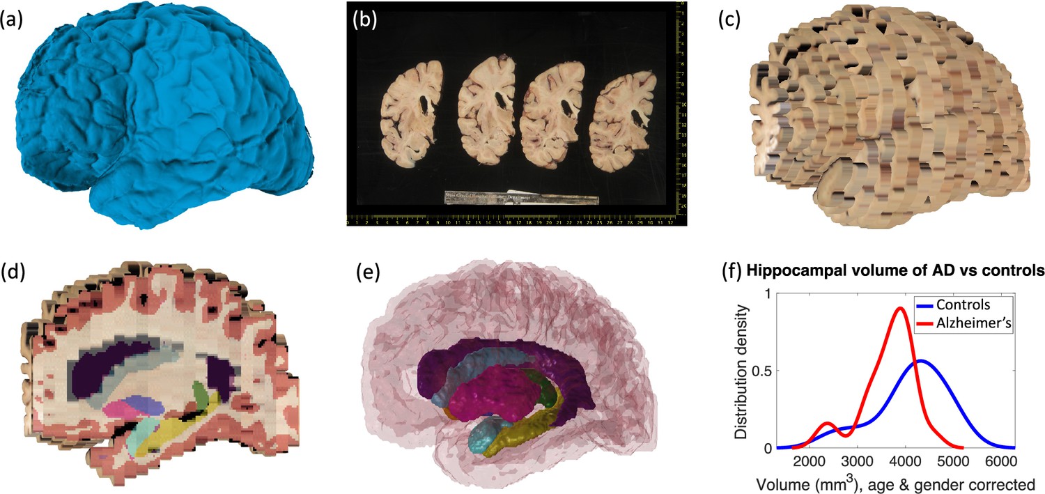
Examples of inputs and outputs from the MADRC dataset.
(a) Three-dimensional (3D) surface scan of left human hemisphere, acquired prior to dissection. (b) Routine dissection photography of coronal slabs, after pixel calibration, with digital rulers overlaid. (c) 3D reconstruction of the photographs into an imaging volume. (d) Sagittal cross-section of the volume in (c) with the machine learning segmentation overlaid. The color code follows the FreeSurfer convention. Also, note that the input has low, anisotropic resolution due to the large thickness of the slices (i.e., rectangular pixels in sagittal view), whereas the 3D segmentation has high, isotropic resolution (squared pixels in any view). (e) 3D rendering of the 3D segmentation into the different brain regions, including hippocampus (yellow), amygdala (light blue), thalamus (green), putamen (pink), caudate (darker blue), lateral ventricle (purple), white matter (white, transparent), and cortex (red, transparent). (f) Distribution of hippocampal volumes in post mortem confirmed Alzheimer’s disease vs controls in the MADRC dataset, corrected for age and gender.
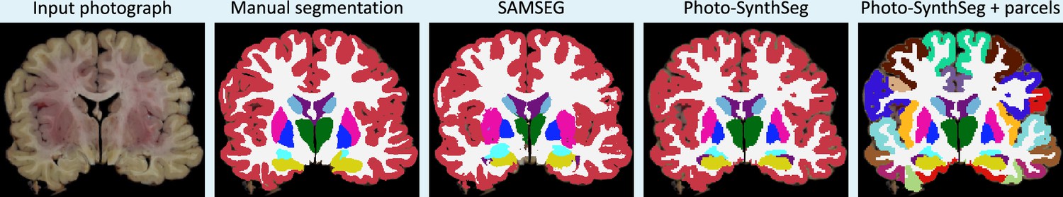
Figure 2
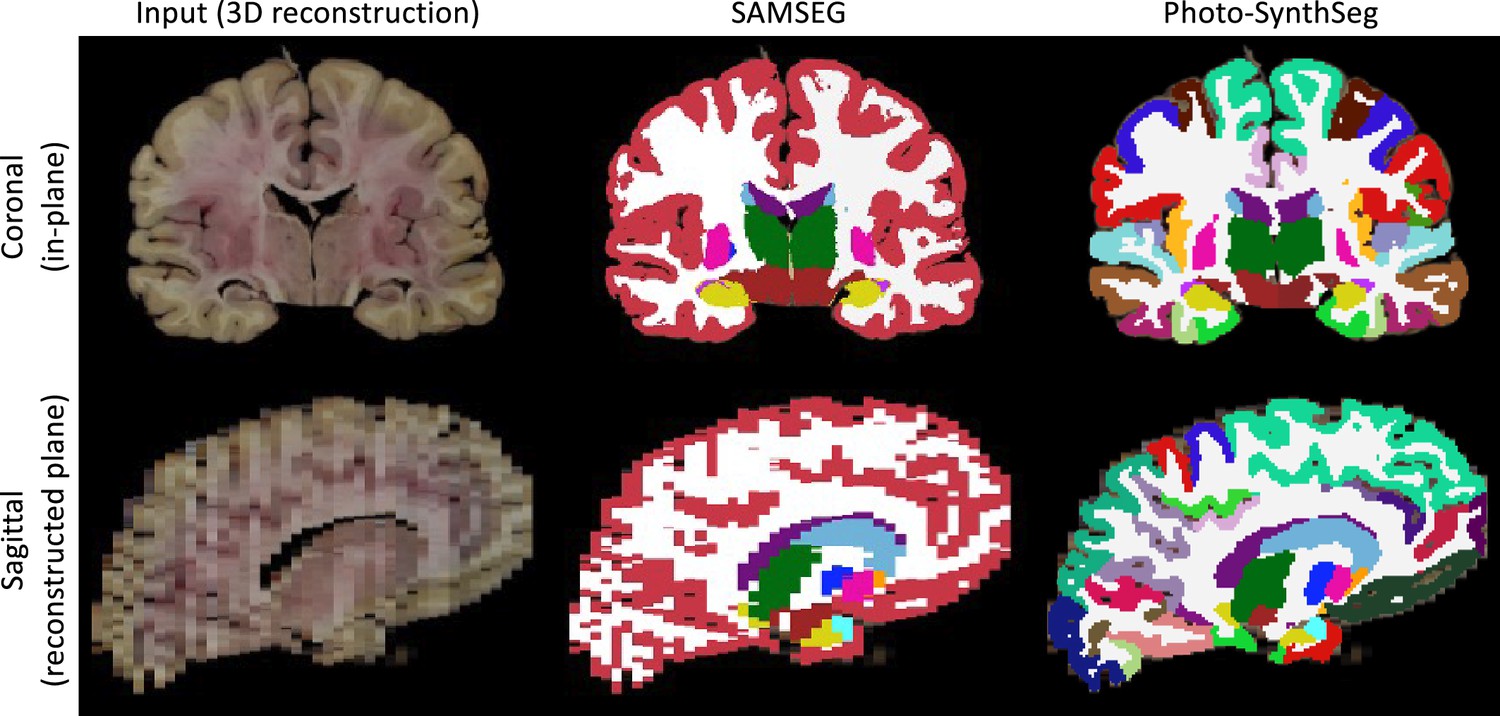
Qualitative comparison of SAMSEG vs Photo-SynthSeg: coronal (top) and sagittal (bottom) views of the reconstruction and automated segmentation of a sample whole brain from the UW-ADRC dataset.
Note that Photo-SynthSeg supports subdivision of the cortex with tools of the SynthSeg pipeline.
Figure 3
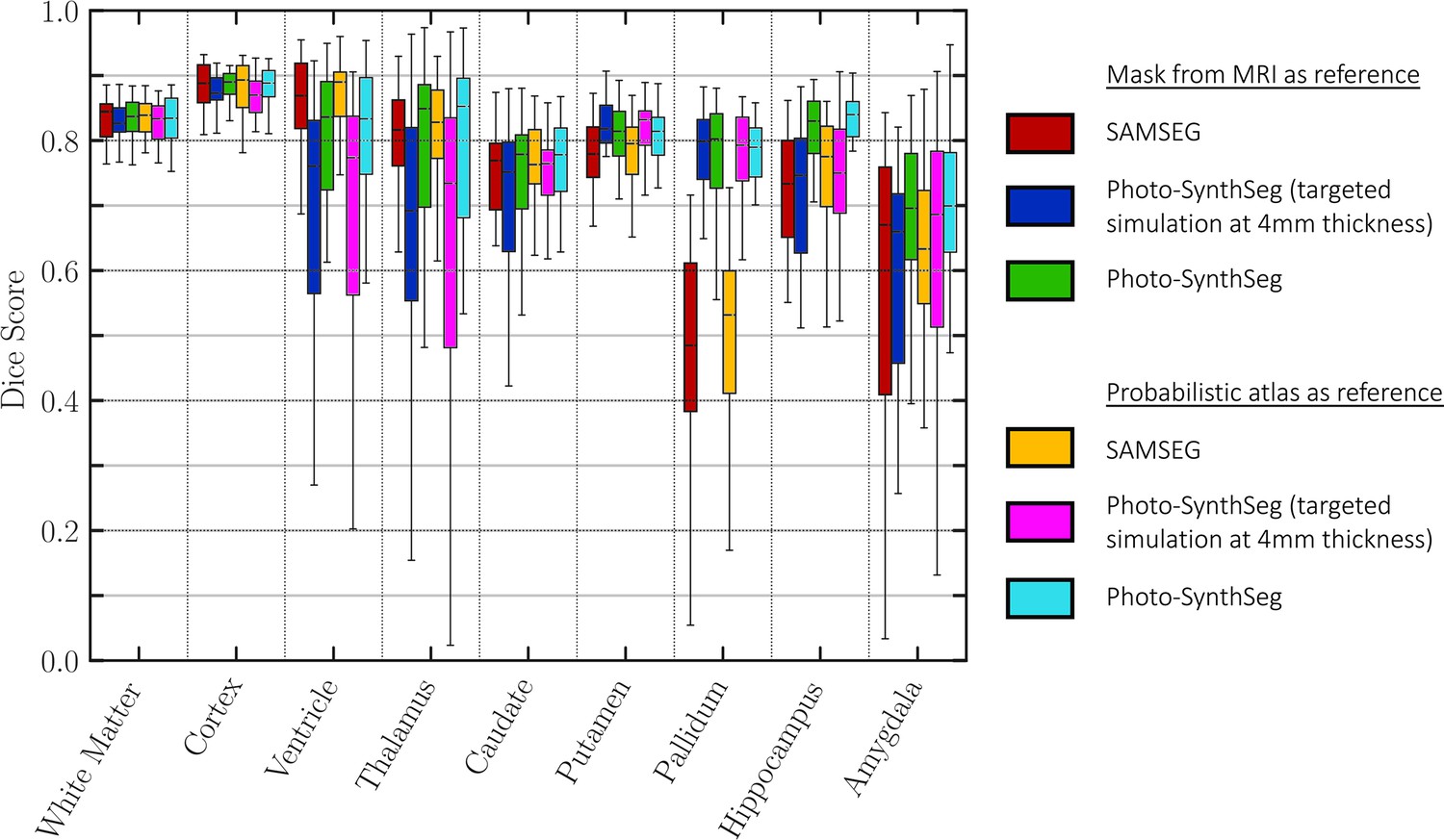
Dice scores of automated vs manual segmentations on select slices.
Box plots are shown for SAMSEG, Photo-SynthSeg, and two ablations: use of probabilistic atlas and targeted simulation with 4 mm slice spacing. Dice is computed in two-dimensional (2D), using manual segmentations on select slices. We also note that the absence of extracerebral tissue in the images contributes to high Dice for the cortex.
Figure 4
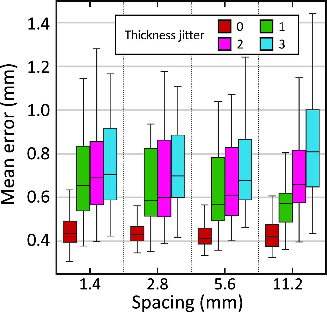
Reconstruction error (in mm) in synthetically sliced HCP data.
The figure shows box plots for the mean reconstruction error as a function of spacing and thickness jitter. A jitter of means that the nth slice is randomly extracted from the interval (rather than exactly ). The center of each box represents the median; the edges of the box represent the first and third quartiles; and the whiskers extend to the most extreme data points not considered outliers (not shown, in order not to clutter the plot).
Figure 5
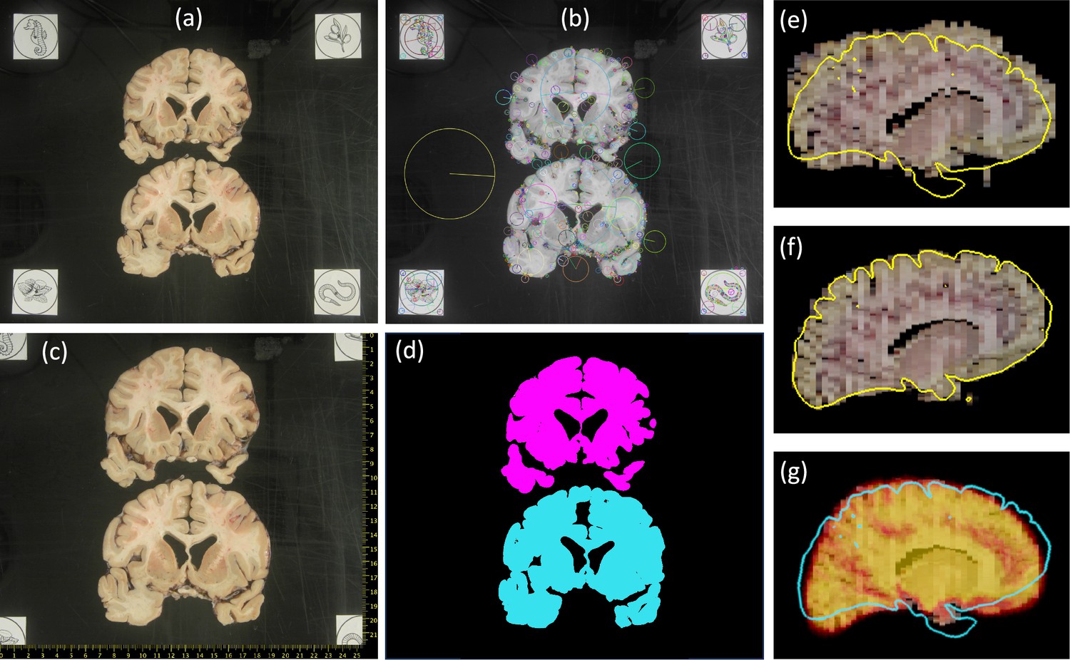
Steps of proposed processing pipeline.
(a) Dissection photograph with brain slices on black board with fiducials. (b) Scale-invariant feature transform (SIFT) features for fiducial detection. (c) Photograph from (a) corrected for pixel size and perspective, with digital ruler overlaid. (d) Segmentation against the background, grouping pieces of tissue from the same slice. (e) Sagittal slice of the initialization of a three-dimensional (3D) reconstruction. (f) Corresponding slice of the final 3D reconstruction, obtained with a surface as reference (overlaid in yellow). (g) Corresponding slice of the 3D reconstruction provided by a probabilistic atlas (overlaid as a heat map); the real surface is overlaid in light blue for comparison.
Figure 6
Intermediate steps in the generative process.
(a) Randomly sampled input label map from the training set. (b) Spatially augmented input label map; imperfect 3D reconstruction is simulated with a deformation jitter across the coronal plane. (c) Synthetic image obtained by sampling from a Gaussian mixture model conditioned on the segmentation, with randomized means and variances. (d) Slice spacing is simulated by downsampling to low resolution. This imaging volume is further augmented with a bias field and intensity transforms (brightness, contrast, gamma). (e) The final training image is obtained by resampling (d) to high resolution. The neural network is trained with pairs of images like (e) (input) and (b) (target).
Appendix 1—figure 1
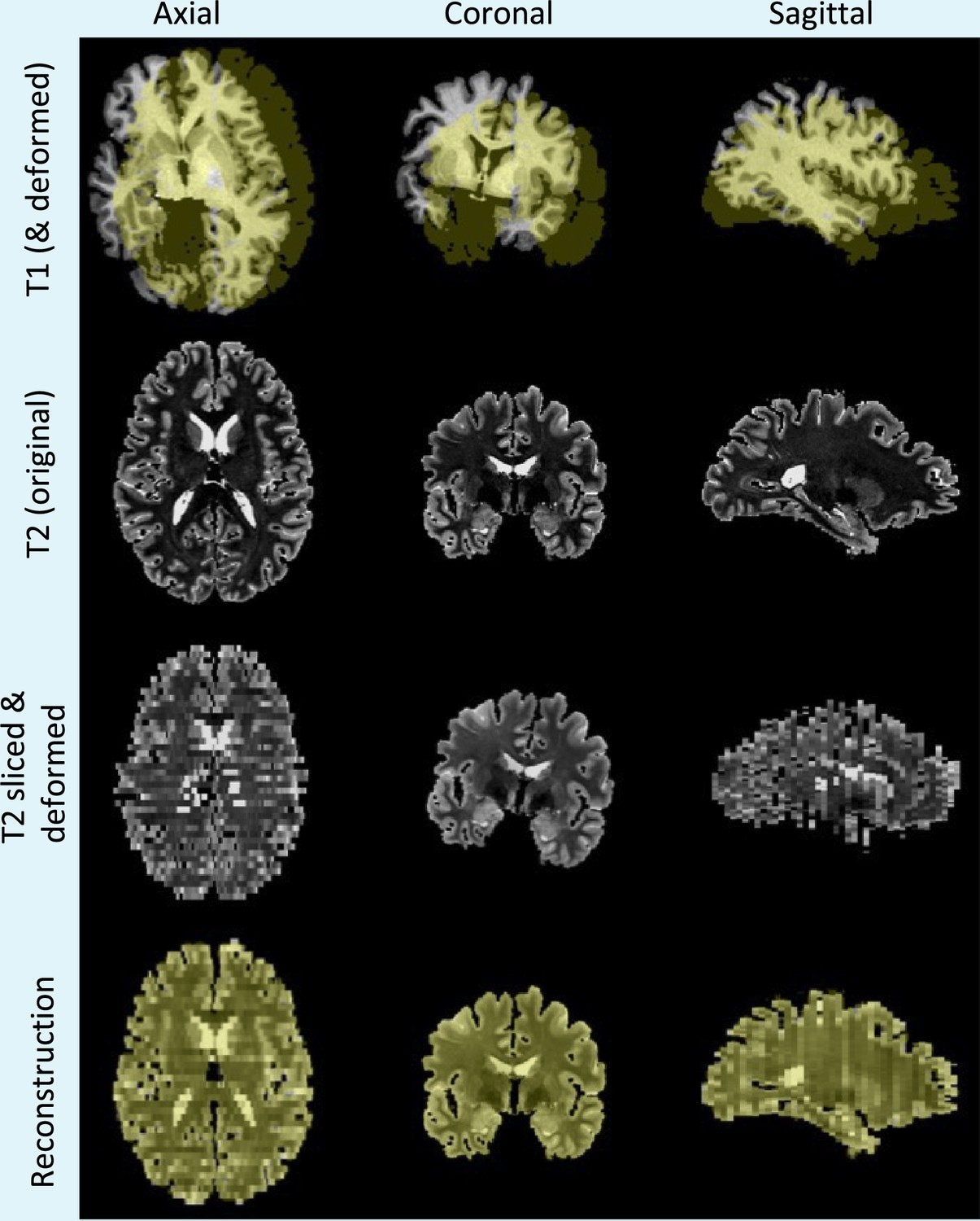
Simulation and reconstruction of synthetic data.
Top row: skull stripped T1 scan and (randomly translated and rotated) binary mask of the cerebrum, in yellow. Second row: original T2 scan. Third row: randomly sliced and linearly deformed T2 images. Bottom row: output of the 3D reconstruction algorithm, that is, reconstructed T2 slices and registered reference mask overlaid in yellow.
Appendix 1—figure 2
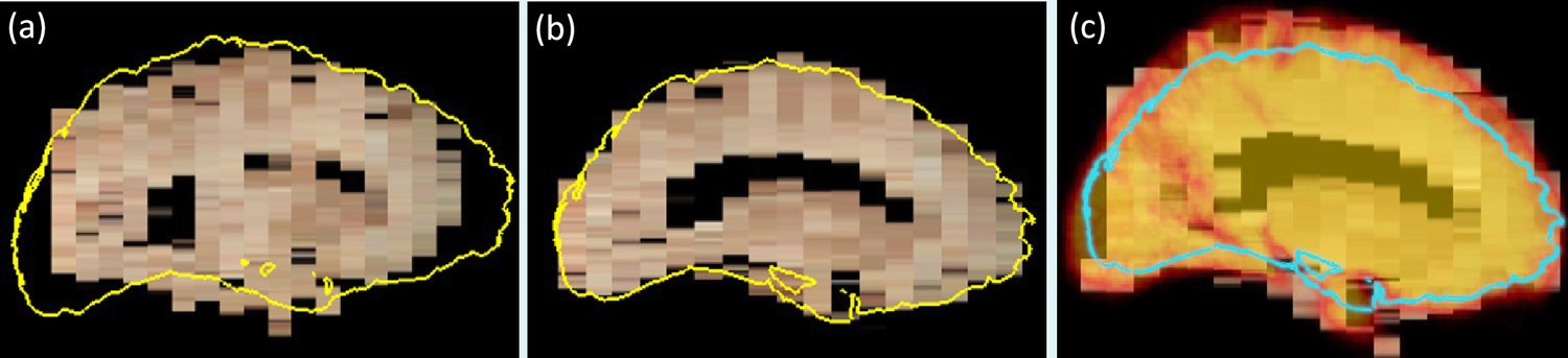
Reconstruction with surface scan vs probabilistic atlas.
(a) Initialization, with contour of 3D surface scan superimposed. (b) Reconstruction with 3D surface scan. (c) Reconstruction with probabilistic atlas (overlaid as heat map with transparency); the contour of the surface scan is overlaid in light blue, for comparison. Even though the shape of the reconstruction in (c) is plausible, it is clearly inaccurate in light of the surface scan.
Appendix 1—figure 3
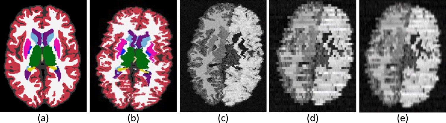
Example of mid-coronal slice selected for manual segmentation and computation of Dice scores.
Compared with the FreeSurFer protocol, we merge the ventral diencephalon (which has almost no visible contrast in the photographs) with the cerebral white matter in our manual delineations. We also merged this structures in the automated segmentations from SAMSEG and Photo-SynthSeg in this figure, for a more consistent comparison.
Videos
Video 1
Overview of the proposed method.
Tables
Table 1
Area under the receiver operating characteristic curve (AUROC) and p-value of a non-parametric Wilcoxon rank sum test comparing the volumes of brain regions for Alzheimer’s cases vs controls.
The volumes were corrected by age and sex using a general linear model. We note that the AUROC is bounded between 0 and 1 (0.5 is chance) and is the non-parametric equivalent of the effect size (higher AUROC corresponds to larger differences). The sample size is .
| Region | Wh matter | Cortex | Vent | Thal | Caud | Putamen | Pallidum | Hippoc | Amyg |
|---|---|---|---|---|---|---|---|---|---|
| AUROC | 0.45 | 0.52 | 0.73 | 0.48 | 0.65 | 0.64 | 0.77 | 0.75 | 0.77 |
| p-value | 0.666 | 0.418 | 0.016 | 0.596 | 0.086 | 0.092 | 0.005 | 0.009 | 0.007 |
Table 2
Correlations of volumes of brains regions estimated by SAMSEG and Photo-SynthSeg from the photographs against the ground truth values derived from the magnetic resonance imaging (MRI).
The p-values are for Steiger tests comparing the correlations achieved by the two methods (accounting for the common sample).
| Mask from MRI as reference | Probabilistic atlas as reference | |||||
|---|---|---|---|---|---|---|
| SAMSEG | Photo-SynthSeg | p-value | SAMSEG | Photo-SynthSeg | p-value | |
| White matter | 0.935 | 0.981 | 0.0011 | 0.886 | 0.935 | 0.0117 |
| Cortex | 0.930 | 0.979 | 0.0001 | 0.889 | 0.920 | 0.0366 |
| Ventricle | 0.968 | 0.988 | 0.0004 | 0.980 | 0.993 | 0.0006 |
| Thalamus | 0.812 | 0.824 | 0.4350 | 0.812 | 0.824 | 0.4252 |
| Caudate | 0.719 | 0.779 | 0.2525 | 0.733 | 0.792 | 0.2062 |
| Putamen | 0.904 | 0.779 | 0.9923 | 0.872 | 0.792 | 0.9598 |
| Pallidum | 0.727 | 0.694 | 0.6171 | 0.676 | 0.658 | 0.5698 |
| Hippocampus | 0.830 | 0.757 | 0.8873 | 0.764 | 0.776 | 0.4293 |
| Amygdala | 0.598 | 0.703 | 0.1663 | 0.576 | 0.763 | 0.0221 |
Additional files
Download links
A two-part list of links to download the article, or parts of the article, in various formats.
Downloads (link to download the article as PDF)
Open citations (links to open the citations from this article in various online reference manager services)
Cite this article (links to download the citations from this article in formats compatible with various reference manager tools)
Machine learning of dissection photographs and surface scanning for quantitative 3D neuropathology
eLife 12:RP91398.
https://doi.org/10.7554/eLife.91398.4


