Modulation of alpha oscillations by attention is predicted by hemispheric asymmetry of subcortical regions
- Centre for Human Brain Health, School of Psychology, University of Birmingham, United Kingdom
- School of Psychology, University of New South Wales, Australia
- CERMEP-Imagerie du Vivant, MEG Department, France
Figures
Figure 1
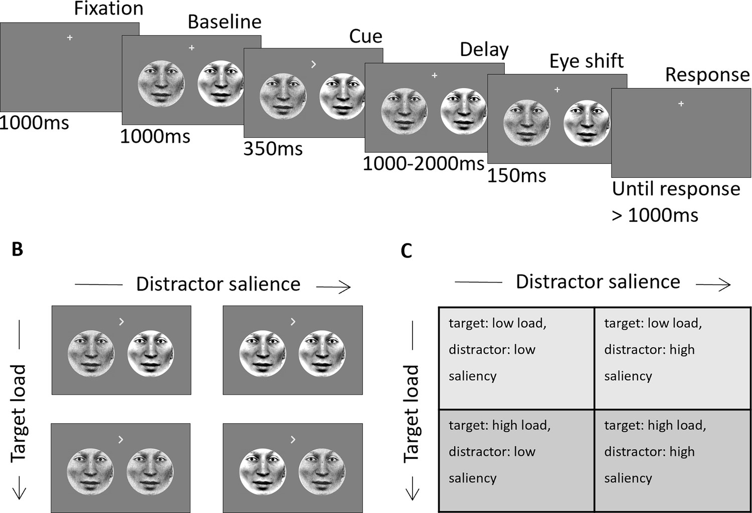
Schematic of experimental design.
(A) Two face stimuli were presented simultaneously in the left and right hemifield. After baseline, a directional cue indicated the location of the target. After a variable delay interval (1000–2000ms) the eye-gaze of each stimulus (independent of the other) shifted randomly to the right or left. Subjects had to indicate the direction of the target eye movement after the delay interval. (B) Examples of visual stimuli for each of the four conditions. (C) Table with the labels of the four load/salience conditions. Adapted from Figure 1 of Gutteling et al., 2022.
Figure 2
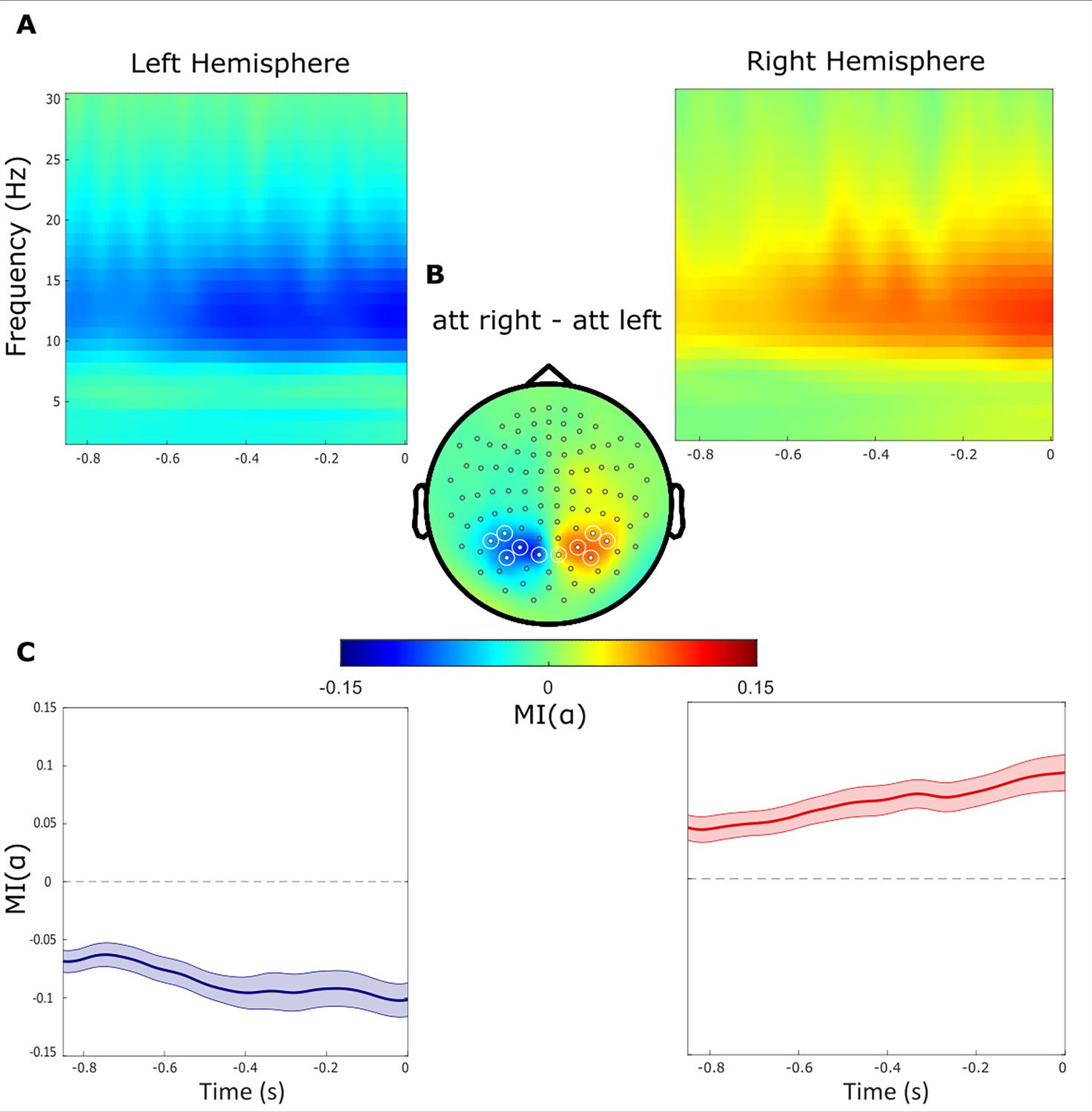
Alpha power decreases contralaterally and increases ipsilaterally with respect to the cued hemifield.
(A) Time-frequency representations of power demonstrate the difference between attended right versus left trials (t=0 indicate the target onset). (B) Topographical plot of the relative difference between attend right versus left trials. Regions of Interest sensors (ROIs) are marked with white circles. (C) The alpha band modulation MI(α) averaged over ROI sensors within the left and right hemispheres, respectively. The absolute MI(α) increased gradually during the delay interval until the onset of the target stimuli.
Figure 3
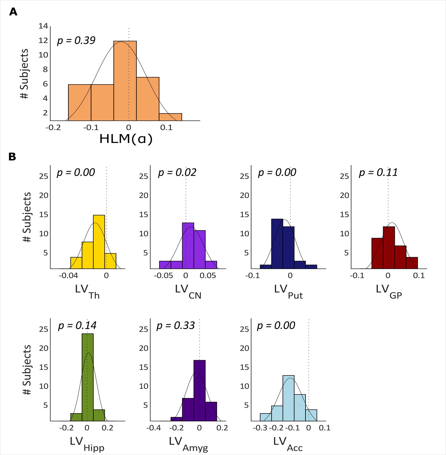
Hemispheric lateralization modulation (HLM(α)) grand average and basal ganglia volumes across all participants.
(A) The HLM(α) distribution across participants. While there was considerable variation across participants, we observed no hemispheric bias in lateralized modulation values across participants (p-value = 0.39). (B) Histograms of the lateralization volumes of subcortical regions. We found that caudate nucleus was right lateralized (p-value = 0.021), whereas, putamen, nucleus accumbens, and thalamus volumes showed left lateralization (p-value = 0.004, p-value <0.001 and p-value <0.001, respectively). Th = Thalamus, CN = Caudate nucleus, Put = Putamen, GP = Globus pallidus, Hipp = Hippocampus, Amyg = Amygdala, Acc = Nucleus accumbens.
Figure 4 with 1 supplement

Lateralization volume of thalamus, caudate nucleus, and globus pallidus in relation to hemispheric lateralization modulation of alpha (HLM(α)) in the task.
(A) The β coefficients for the best model (containing three regressors) associated with a generalized linear model (GLM) where lateralization volume (LV) values were defined as explanatory variables for HLM(α). The model significantly explained the HLM(α) (p-value = 0.0007). Error bars indicate standard errors of mean (SEM), n = 33. Asterisks denote statistical significance; *p-value <0.05. (B) Partial regression plot showing the association between LVTh and HLM(α) while controlling for LVGP and LVCN (p-value = 0.01). (C) Partial regression plot showing the association between LVGP and HLM(α) while controlling for LVTh and LVCN (p-value = 0.061). (D) Partial regression plot showing the association between LVCN and HLM(α) while controlling for LVTh and LVGP (p-value = 0.008). Negative (or positive) LVs indices denote greater left (or right) volume for a given substructure; similarly negative HLM(α) values indicate stronger modulation of alpha power in the left compared with the right hemisphere, and vice versa. The dotted curves in B, C, and D indicate 95% confidence bounds for the regression line fitted on the plot in red.
Figure 4—figure supplement 1
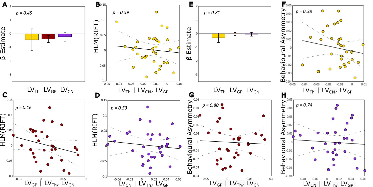
Lateralization volume of thalamus, caudate nucleus, and globus pallidus in relation to hemispheric lateralization modulation of rapid invisible frequency tagging (HLM(RIFT)) on the right and behavioural asymmetry on the left.
(A and E) The β coefficients for the best model (having three regressors) associated with a generalized linear model (GLM) where lateralization volume (LV) values were defined as explanatory variables for HLM(RIFT) (A) and behavioural asymmetry (E). Error bars indicate standard errors of mean (SEM), n = 33. (B and F) Partial regression plot showing the association between LVTh and HLM(RIFT) (B, p-value = 0.59) and behavioural asymmetry (F, p-value = 0.38) while controlling for LVGP and LVCN. (C and G), Partial regression plot showing the association between LVGP and HLM(RIFT) (C, p-value = 0.16) and behavioural asymmetry (G, p-value = 0.80) while controlling for LVTh and LVCN. (D and H) Partial regression plot showing the association between LVCN and HLM(RIFT) (D, p-value = 0.53) and behavioural asymmetry (H, p-value = 0.74) while controlling for LVTh and LVGP. Negative (or positive) LVs indices denote greater left (or right) volume for a given substructure; similarly negative HLM(RIFT) values indicate stronger modulation of RIFT power in the left compared with the right hemisphere, and vice versa; positive behavioural asymmetry value shows higher accuracy when the target was on the right as compared with left, and vice versa for negative behavioural asymmetry values. The dotted curves in (B, C, D, F, G, and H) indicate 95% confidence bounds for the regression line fitted on the plot in red.
Figure 5

β estimates of subcortical nuclei from a multivariate regression model predicting HLM(α) in the four perceptual load conditions.
Here, the HLM(α) values for the four load conditions are the dependent variables and the lateralization volume of subcortical structures are the explanatory variables. The model significantly explains HLM(α) variability (p-value = 0.001) in comparison with null model. Error bars indicate SEM, n = 33. Asterisks denote statistical significance; *p-value <0.05.
Author response image 1

Author response image 2

Tables
Author response table 1
| Regression | Comb. 1 | Comb. 2 | Comb. 3 | Comb. 4 | Comb. 5 | Comb. 6 | Comb. 7 | Comb. 8 | Comb. 9 | Comb. 10 | Comb. 11 | Comb. 12 | Comb. 13 | Comb. 14 | Comb. 15 | Comb. 16 | Comb. 17 | Comb. 18 | Comb. 19 | Comb. 20 | Comb. 21 | Model criterion |
|---|---|---|---|---|---|---|---|---|---|---|---|---|---|---|---|---|---|---|---|---|---|---|
| –81.63 | –77.78 | –73.75 | –78.62 | –71.94 | –73.18 | –71.48 | NaN | NaN | NaN | NaN | NaN | NaN | NaN | NaN | NaN | NaN | NaN | NaN | NaN | NaN | AIC | |
| –77.33 | –73.48 | –69.45 | –74.32 | –67.64 | –68.88 | –67.18 | NaN | NaN | NaN | NaN | NaN | NaN | NaN | NaN | NaN | NaN | NaN | NaN | NaN | NaN | BIC | |
| –86.72 | –79.93 | –82.66 | –77.88 | –78.04 | –78.00 | –76.42 | –81.27 | –75.82 | –75.83 | –73.89 | –77.41 | –70.41 | –71.36 | –69.94 | –74.79 | –76.05 | –74.63 | –70.08 | –68.23 | –69.30 | AIC | |
| –81.11 | –74.32 | –77.05 | –72.28 | –72.44 | –72.39 | –70.82 | –75.66 | –70.22 | –70.23 | –68.29 | –71.81 | –64.81 | –65.75 | –64.33 | –69.19 | –70.44 | –69.03 | –64.48 | –62.63 | –63.70 | BIC | |
| –85.30 | –87.54 | –82.79 | –82.96 | –82.64 | –81.00 | –76.18 | –76.19 | –76.29 | –78.86 | –79.00 | –78.73 | –74.25 | –74.24 | –74.32 | –79.67 | –74.61 | –74.06 | –72.55 | –78.51 | –78.88 | AIC | |
| –78.46 | –80.71 | –75.95 | –75.13 | –75.81 | –74.17 | –69.34 | –69.35 | –69.46 | –72.02 | –72.17 | –71.90 | –67.42 | –57.40 | –67.49 | –72.84 | –67.77 | –67.22 | –65.72 | –71.68 | –72.05 | BIC | |
| –85.52 | –81.42 | –81.27 | –81.21 | –83.50 | –83.73 | –83.30 | –79.33 | –78.80 | –78.85 | –77.26 | –77.72 | –77.09 | –72.43 | –72.54 | –72.49 | –75.15 | –74.95 | –75.04 | –70.57 | –76.78 | AIC | |
| –77.52 | –73.43 | –73.28 | –73.21 | –75.50 | –75.74 | –75.31 | –71.33 | –70.80 | –70.86 | –69.27 | –69.73 | –69.10 | –64.44 | –64.55 | –64.45 | –67.15 | –66.96 | –67.04 | –62.58 | –68.78 | BIC | |
| –81.51 | –81.90 | –81.30 | –77.65 | –77.41 | –77.17 | –79.95 | –79.32 | –79.49 | –75.29 | –73.88 | –73.36 | –73.75 | –68.77 | –71.22 | –75.31 | –72.78 | –73.87 | –68.85 | –72.63 | –67.74 | AIC | |
| –72.44 | –72.83 | –72.24 | –68.58 | –68.34 | –68.01 | –70.88 | –70.25 | –70.42 | –66.22 | –64.81 | –64.29 | –64.68 | –59.70 | –62.15 | –66.24 | –63.71 | –64.79 | –59.78 | –63.56 | –58.67 | BIC | |
| –78.13 | –77.37 | –77.70 | –73.63 | –75.76 | –69.96 | –71.25 | NaN | NaN | NaN | NaN | NaN | NaN | NaN | NaN | NaN | NaN | NaN | NaN | NaN | NaN | AIC | |
| –68.07 | –67.30 | –67.63 | –63.56 | –65.70 | –59.89 | –61.19 | NaN | NaN | NaN | NaN | NaN | NaN | NaN | NaN | NaN | NaN | NaN | NaN | NaN | NaN | BIC | |
| –74.00 | NaN | NaN | NaN | NaN | NaN | NaN | NaN | NaN | NaN | NaN | NaN | NaN | NaN | NaN | NaN | NaN | NaN | NaN | NaN | NaN | AIC | |
| –63.01 | NaN | NaN | NaN | NaN | NaN | NaN | NaN | NaN | NaN | NaN | NaN | NaN | NaN | NaN | NaN | NaN | NaN | NaN | NaN | NaN | BIC |
Author response table 2
| Regre ssion | Com b. 22 | Com b. 23 | Com b. 24 | Com b. 25 | Com b. 26 | Com b. 27 | Com b. 28 | Com b. 29 | Com b. 30 | Com b. 31 | Com b. 32 | Com b. 33 | Com b. 34 | Com b. 35 | Mo del crite rion |
|---|---|---|---|---|---|---|---|---|---|---|---|---|---|---|---|
| HLM∼,beta_(LV_(1)) | NaN | NaN | NaN | NaN | NaN | NaN | NaN | NaN | NaN | NaN | NaN | NaN | NaN | NaN | bar(" AIC ") |
| NaN | NaN | NaN | NaN | NaN | NaN | NaN | NaN | NaN | NaN | NaN | NaN | NaN | NaN | BIC | |
| HLM∼,beta_(LV_(1))+,beta_(LV_(2)) | NaN | NaN | NaN | NaN | NaN | NaN | NaN | NaN | NaN | NaN | NaN | NaN | NaN | NaN | AIC |
| NaN | NaN | NaN | NaN | NaN | NaN | NaN | NaN | NaN | NaN | NaN | NaN | NaN | NaN | BIC | |
| HLM beta_(LV_(1))+,beta_(LV_(2))+,beta_(LV_(3)) | 77.3 | 74.5,9 | 71.9 0 | 71.9,3 | 73.5,4 | 75.4 | 73.4 5 | 68.2 7 | 66.7 | 67.5 | 72.4 0 | 70.8,9 | 72.0 5 | 66.3 | AIC |
| 70.5,0 | 67.7,5 | 65.0,7 | 65.0,9 | 66.7,1 | 68.5,9 | 66.6 | 61.4,3 | 59.8 9 | 60.6,7 | 65.5,7 | 64.0,5 | 65.2 | 59.4,8 | BIC | |
| HLM∼,beta_(LV_(1))+,beta_(LV_(2))+,beta_(LV_(3))+,beta_(LV_(4)) | 77.7 6 | 75.7,6 | 72.8,3 | 70.6 9 | 70.1 9 | 76.7,2 | 74.4 | 74.9 7 | 70.5,8 | 71.6 7 | 69.6 6 | 71.4 | 64.5,3 | 68.4 | AIC |
| 69.7,6 | 67.7,7 | 64.8,4 | 62.7 0 | 62.1,9 | 68.7 | 66.4,9 | 66.9,8 | 62.5,9 | 63.6,8 | 61.6,7 | 63.4 | 56.5,3 | 60.4 7 | BIC | |
| HLM beta_(LV_(1))+,beta_(LV_(2))+,beta_(LV_(3))+,beta_(LV_(4))+,beta_(LV_(3)) | NaN | NaN | NaN | NaN | NaN | NaN | NaN | NaN | NaN | NaN | NaN | NaN | NaN | NaN | AIC |
| NaN | NaN | NaN | NaN | NaN | NaN | NaN | NaN | NaN | NaN | NaN | NaN | NaN | NaN | BIC | |
| HLM beta_(LV_(1))+,beta_(LV_(2))+,beta_(LV_(3))+,beta_(LV_(4))+,beta_(LV_(5))+,beta_(LV_(n)) | NaN | NaN | NaN | NaN | NaN | NaN | NaN | NaN | NaN | NaN | NaN | NaN | NaN | NaN | AIC |
| NaN | NaN | NaN | NaN | NaN | NaN | NaN | NaN | NaN | NaN | NaN | NaN | NaN | NaN | BIC | |
| HLM beta_(LV_(1))+,beta_(LV_(2))+,beta_(LV_(3))+,beta_(LV_(4))+,beta_(LV_(5))+,beta_(LV_(6))+,beta_(LV_(-)) | NaN | NaN | NaN | NaN | NaN | NaN | NaN | NaN | NaN | NaN | NaN | NaN | NaN | NaN | AIC |
| NaN | NaN | NaN | NaN | NaN | NaN | NaN | NaN | NaN | NaN | NaN | NaN | NaN | NaN | BIC |
Author response table 3
Bayes factors for correlation between hemispheric laterality of subcortical structures with hemispheric lateralization modulation of rapid invisible frequency tagging (HLM(RIFT)) and with behavioural asymmetry (BA).
The Pearson correlation between each subcortical structure with HLM(RIFT) and behavioural asymmetry was calculated. The likelihood of the data under the alternative hypothesis (the evidence of correlation) were subsequently compared to the likelihood under null hypothesis (absence of correlation), given the data. As it is demonstrated in the table, all Bayes factors were below or very close to 1 indicating evidence for the null hypothesis.
| Subcortical structure | HLM(RIFT) | BA |
|---|---|---|
| Thalamus | 0.14 | 0.20 |
| Caudate Nucleus | 0.18 | 0.15 |
| Putamen | 0.14 | 0.14 |
| Globus Pallidus | 0.34 | 0.13 |
| Hippocampus | 0.19 | 0.25 |
| Amygdala | 0.54 | 1.18 |
| Nucleus Accumbens | 0.16 | 0.17 |
Additional files
-
Supplementary file 1
Akaike Information Criterion (AIC) and Bayesian Information Criterion (BIC) values for all possible combinations of regressors (Lateralized Volume of subcortical structures).
The selected model, with lowest AIC, is marked in green.
- https://cdn.elifesciences.org/articles/91650/elife-91650-supp1-v1.docx
-
Supplementary file 2
The combination of structures for each regression model above.
The selected model is marked in green.
- https://cdn.elifesciences.org/articles/91650/elife-91650-supp2-v1.docx
-
Supplementary file 3
Bayes factors for correlation between hemispheric laterality of subcortical structures with hemispheric lateralization modulation of rapid invisible frequency tagging (HLM(RIFT)) and with behavioural asymmetry (BA).
The Pearson correlation between each subcortical structure with HLM(RIFT) and behavioural asymmetry was calculated. The likelihood of the data under the alternative hypothesis (the evidence of correlation) were subsequently compared to the likelihood under null hypothesis (absence of correlation), given the data. As it is demonstrated in the table, all Bayes factors were below or very close to 1 indicating evidence for the null hypothesis.
- https://cdn.elifesciences.org/articles/91650/elife-91650-supp3-v1.docx
-
MDAR checklist
- https://cdn.elifesciences.org/articles/91650/elife-91650-mdarchecklist1-v1.pdf
Download links
A two-part list of links to download the article, or parts of the article, in various formats.
Downloads (link to download the article as PDF)
Open citations (links to open the citations from this article in various online reference manager services)
Cite this article (links to download the citations from this article in formats compatible with various reference manager tools)
Modulation of alpha oscillations by attention is predicted by hemispheric asymmetry of subcortical regions
eLife 12:RP91650.
https://doi.org/10.7554/eLife.91650.3


