Reconfigurations of cortical manifold structure during reward-based motor learning
- Centre for Neuroscience Studies, Queen’s University, Canada
- Department of Psychology, Queen’s University, Canada
- Department of Medicine, Queen's University, Canada
- Department of Biomedical and Molecular Sciences, Queen’s University, Canada
Figures
Figure 1 with 2 supplements
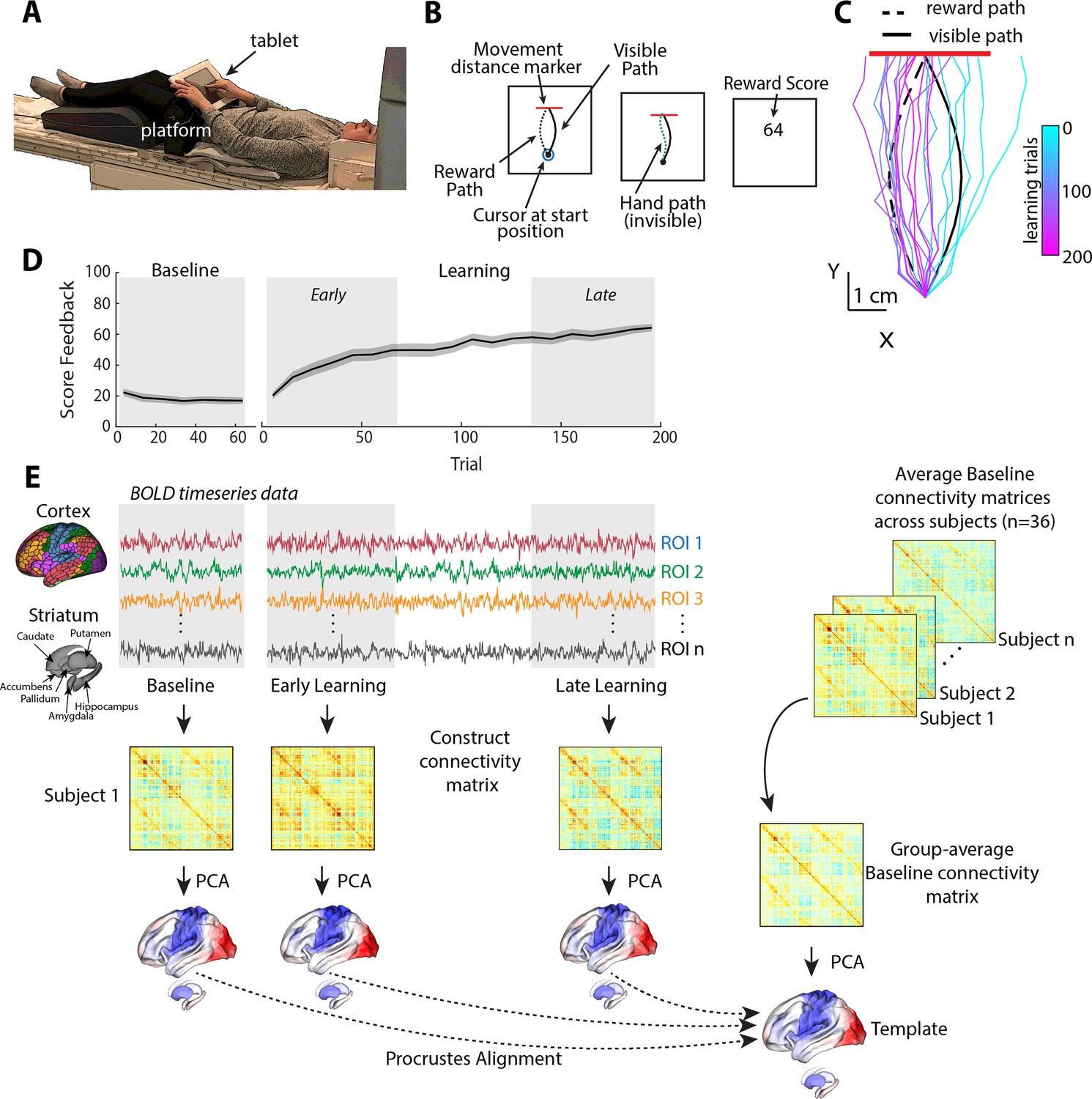
Task structure and overview of fMRI analysis.
(A) Subject setup in the MRI scanner. (B) Trial structure of the reward-based motor learning task. On each trial, subjects were required to trace a curved (Visible) path from a start location to a target line (in red), without visual feedback of their finger location. Following a baseline block of trials, subjects were instructed that they would receive score feedback, presented at the end of the trial, based on their accuracy in tracing the visible path. However, unbeknownst to subjects, the score they received was actually based on how accurately they traced the mirror-image path (reward path), which was invisible to participants. (C) Example subject data from learning trials in the task. Colored traces show individual trials over time (each trace is separated by ten trials to give a sense of the trajectory changes over time; 20 trials shown in total). (D) Average participant performance throughout the learning task. Black line denotes the mean across participants whereas the gray banding denotes ±1 standard error of the mean (SEM). Three equal-length task epochs for subsequent neural analyses are indicated by the gray shaded boxes. (E) Neural analysis approach. For each participant and each task epoch (baseline, early, and late learning), we estimated functional connectivity matrices using region-wise time series extracted from the Schaefer 1000 cortical parcellation and the Harvard-Oxford striatal parcellation. We estimated functional connectivity manifolds for each task epoch using principal component analysis (PCA) with centered and thresholded connectivity matrices (see ‘Materials and methods’, as well as Figure 2). All manifolds were aligned to a common template manifold created from a group-average baseline connectivity matrix (right) using Proscrustes alignment. This allowed us to assess learning-related changes in manifold structure from this baseline architecture.
Figure 1—figure supplement 1
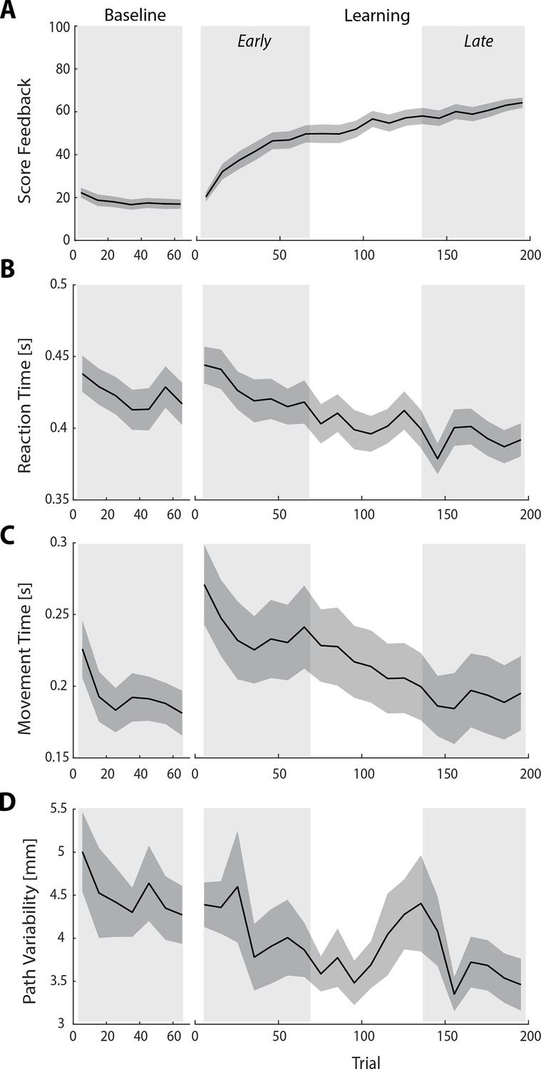
Behavioral measures of learning across the task.
(A–D) show average participant reward scores (A), reaction times (B), movement times (C), and path variability (D) over the course of the task. In each plot, the black line denotes the mean across participants (N=36) and the gray banding denotes ±1 standard error of the mean (SEM). The three equal-length task epochs for subsequent neural analyses are indicated by the gray shaded boxes.
Figure 1—figure supplement 2
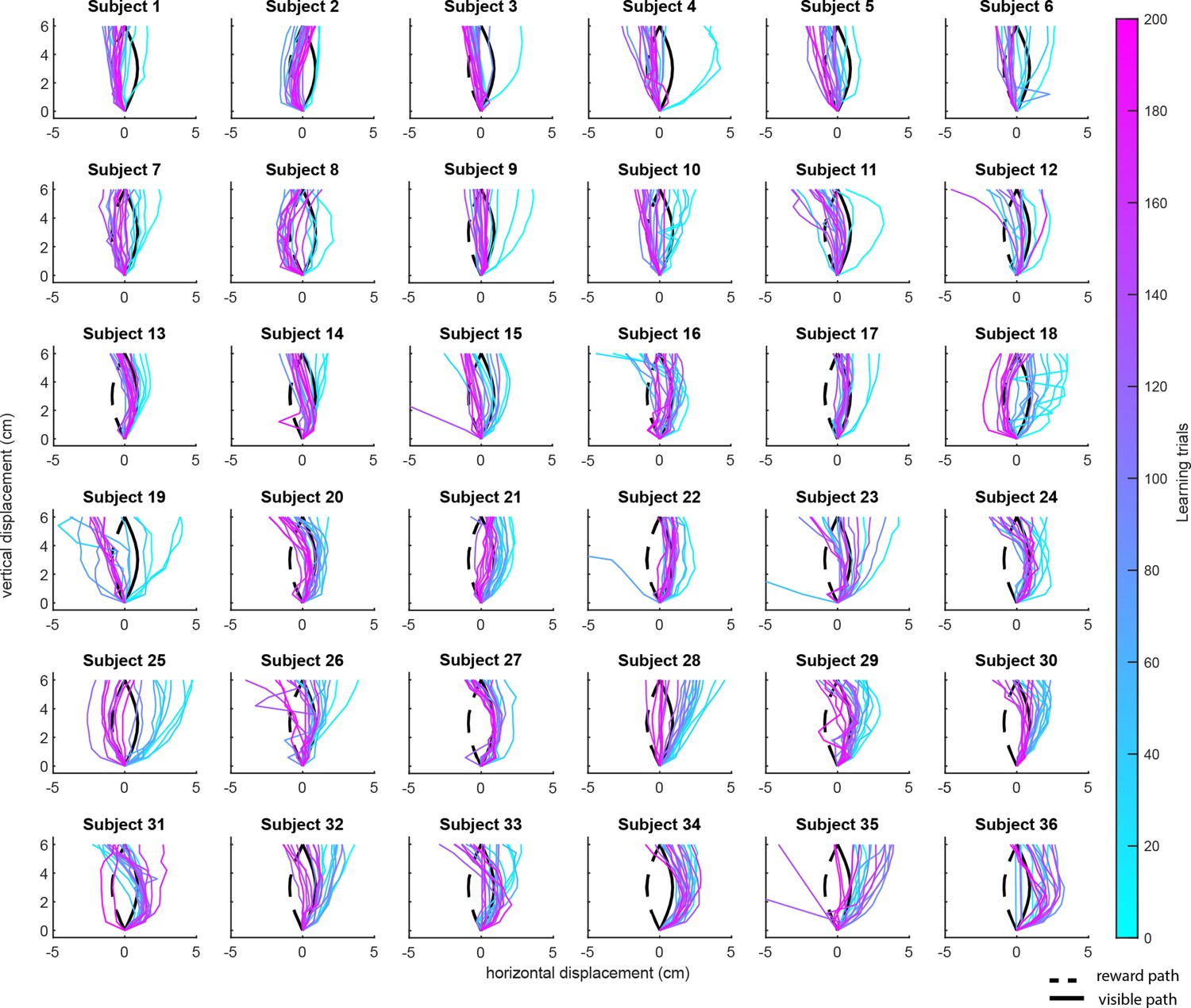
Variability in learning across subjects.
Plots show representative trajectory data from each subject (n = 36) over the course of the 200 learning trials. Colored traces show individual trials over time (each trace is separated by 10 trials, e.g., trial 1, 10, 20, 30, etc.) to give a sense of the trajectory changes throughout the task (20 trials in total are shown for each subject).
Figure 2 with 1 supplement
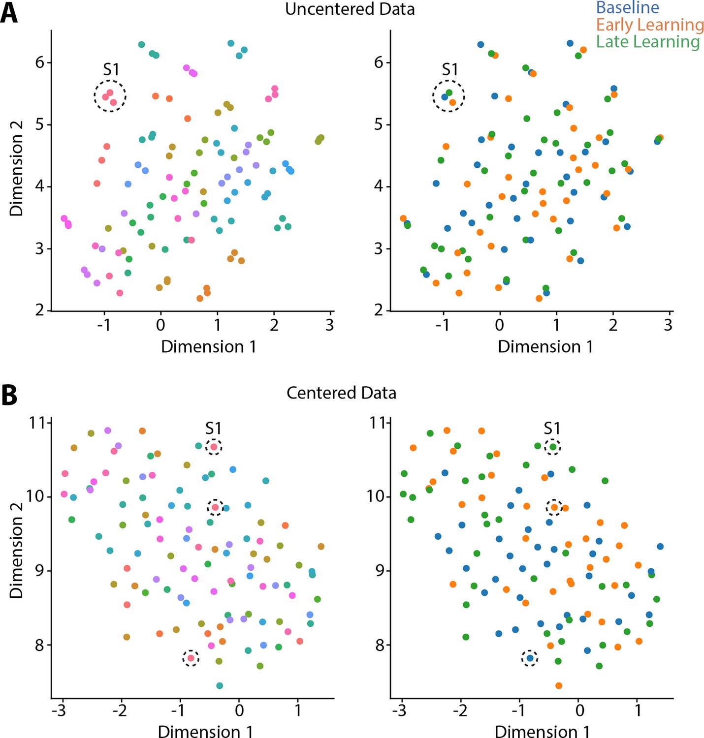
Riemmanian centering removes subject-level clustering.
Uniform Manifold Approximation (UMAP) visualization of the similarity of connectivity matrices, both before centering (A) and after (B) centering. In these plots, each point represents a single functional connectivity matrix, color-coded either to subject identity (left panels) or task epoch (right panels), with its location in the multidimensional space based on the similarity between matrices. Note that the uncentered connectivity matrices in (A) show a high degree of subject-level clustering, thus obscuring any differences in task structure. By contrast, the Riemmanian manifold centering approach (in B) abolishes this subject-level clustering. To help illustrate this point, the dashed circles in both (A) and (B) indicate the functional connectivity matrices belonging to the same single subject (subject 1; S1).
Figure 2—figure supplement 1
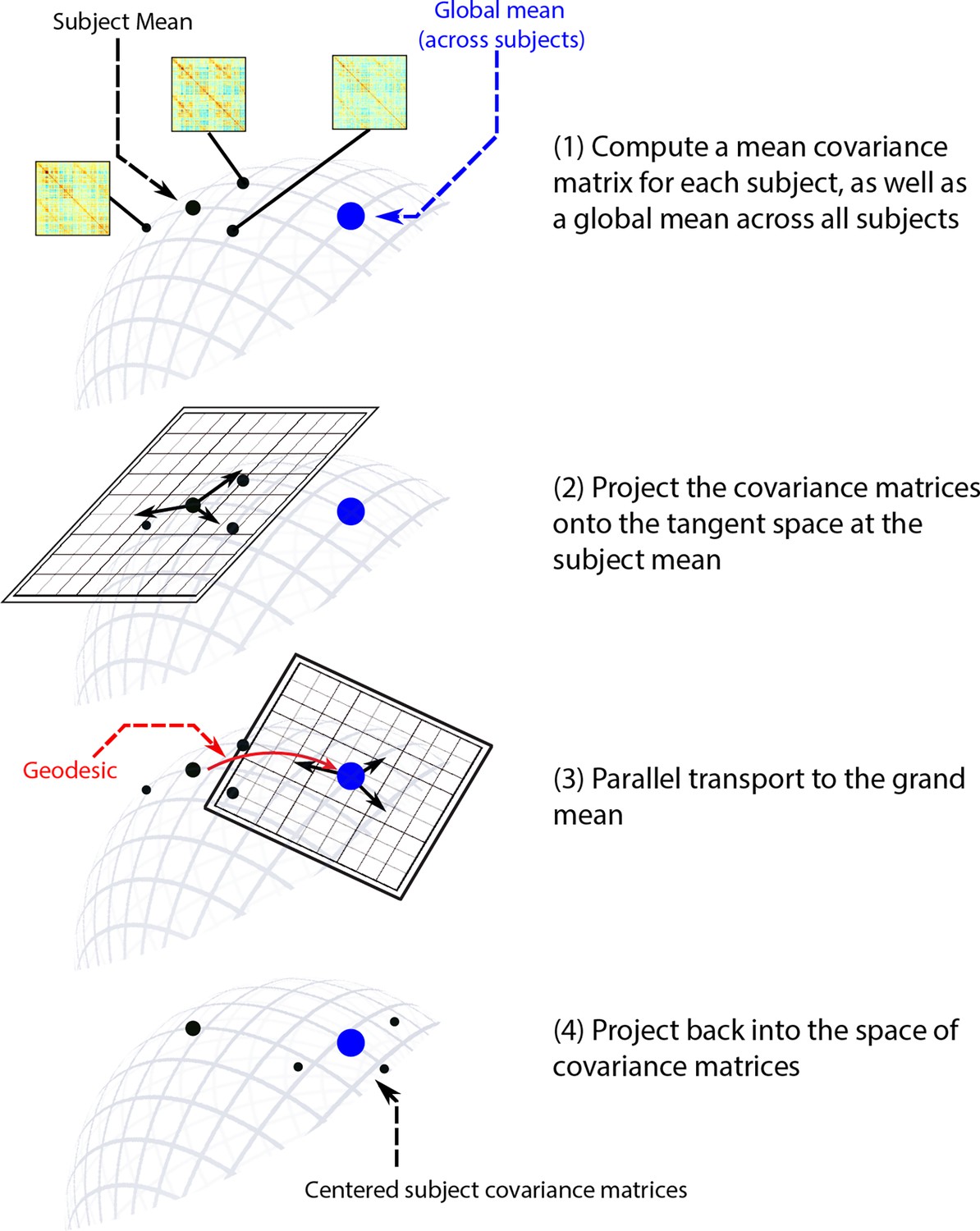
Overview of the Riemannian manifold centering approach.
To minimize the impact of significant individual variations in functional connectivity that might mask task-related changes, we used a Riemannian manifold approach to center all connectivity matrices. See steps #1–4 above for an overview. In short, each participant’s covariance matrices were adjusted to share a common mean (equal to the overall mean covariance) to eliminate static individual differences that could potentially conceal task-related differences in functional connectivity. Since the space of covariance matrices is non-Euclidean, this adjustment cannot be achieved by simple subtraction. Instead, it requires calculating the difference between each covariance matrix and the corresponding participant mean (formally, a tangent vector) and then transporting this tangent vector to the overall grand mean to obtain a new covariance matrix that deviates from the grand mean in a comparable manner. For detailed computations involved in this process, please refer to the corresponding Methods section.
Figure 3 with 2 supplements
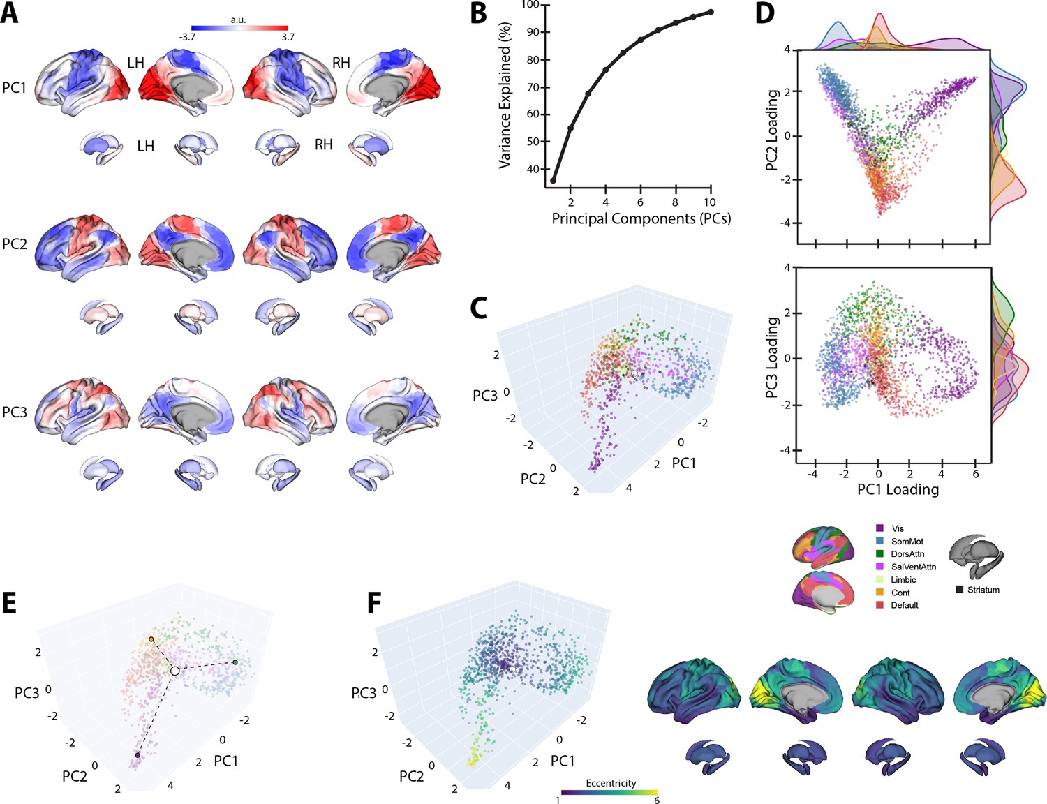
Baseline manifold structure and eccentricity.
(A) Region loadings for the top three principal components (PCs). (B) Percent variance explained for the first 10 PCs. (C) The baseline (template) manifold in low-dimensional space, with regions colored according to functional network assignment (Schaefer et al., 2018; Thomas Yeo et al., 2011). (D) Scatter plots showing the embedding of each region along the top three PCs. Probability density histograms at the top and right show the distribution of each functional network along each PC. Vis: visual; SomMot: somatomotor; DorsAttn: dorsal attention; SalVentAttn: salience/ventral attention; Cont: control. (E) Illustration of how eccentricity is calculated. Region eccentricity along the manifold is computed as the Euclidean distance (dashed line) from manifold centroid (white circle). The eccentricity of three example brain regions is highlighted (bordered colored circles). (F) Regional eccentricity during baseline. Each brain region’s eccentricity is color-coded in the low-dimensional manifold space (left) and on the cortical and striatal surfaces (right). White circle with black bordering denotes the center of the manifold (manifold centroid).
Figure 3—figure supplement 1
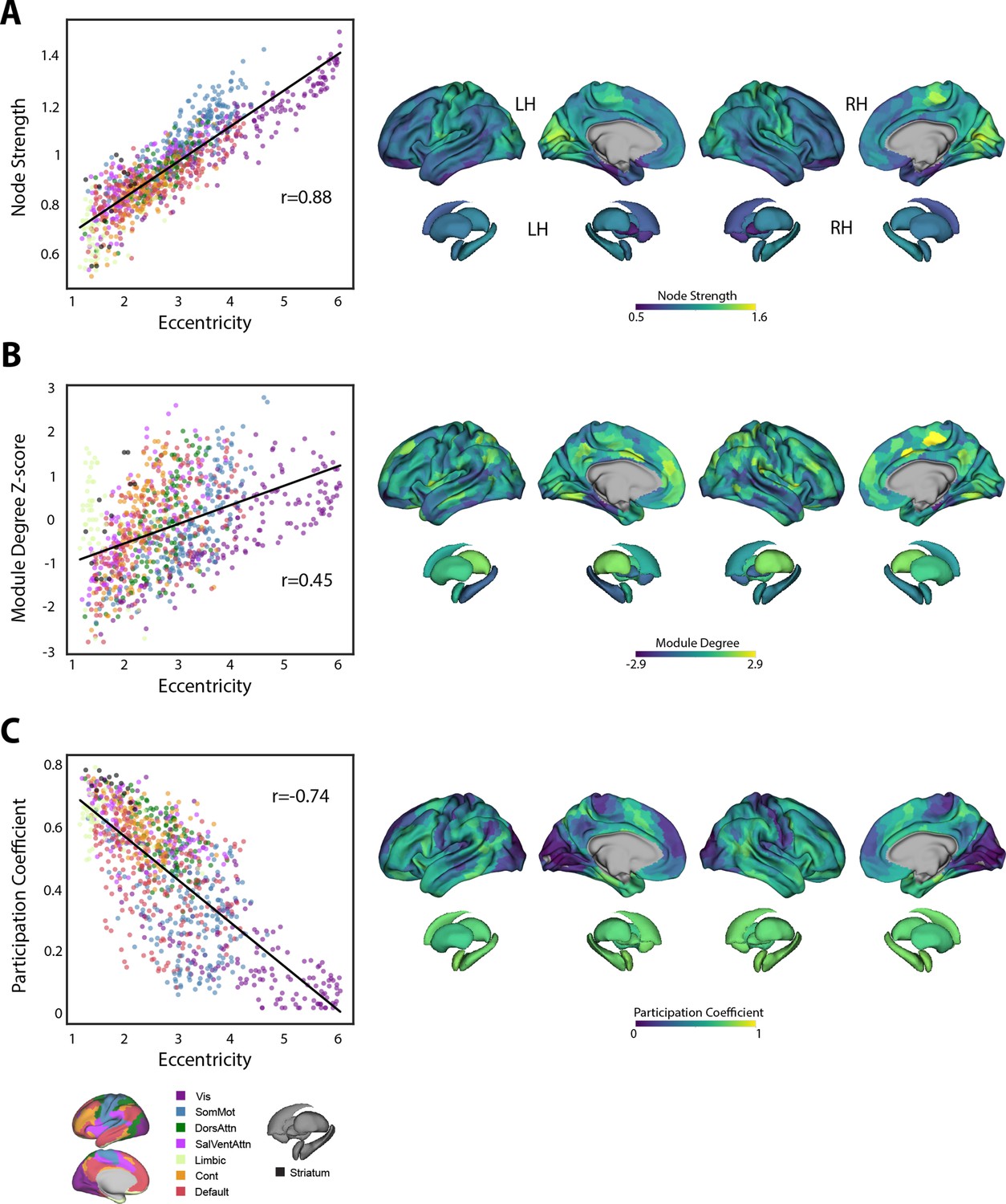
Functional connectivity properties that underlie manifold eccentricity.
(A–C) Different network properties of individual brain areas (derived from functional connectivity) and their correspondence to regional eccentricity. Left: scatterplots show the relationship between each functional connectivity measure and manifold eccentricity, with the line depicting a regression line of best fit to the cortical and striatal data. Right: brain plots show the maps of node strength, within-module degree z-score and participation coefficient, derived from the group-average baseline connectivity matrix (i.e., reference connectivity matrix).
Figure 3—figure supplement 2
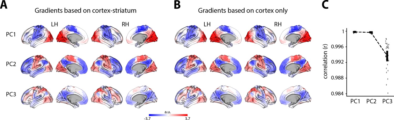
Derivation of cortical gradients did not depend on the inclusion of the striatum in the analysis.
(A) Principal components (PCs) 1–3 based on principal components analysis (PCA) decomposition of the group-average template baseline functional connectivity matrix, which included both cortical and striatal regions (as in Figure 3A). (B) Same as in (A), but based on a group-average template baseline functional connectivity matrix that did not include the striatal regions. (C) Whole-brain Pearson correlations between the data from (A) and (B), for each PC. Vertical lines denote the mean ±1 SEM. Single data points denote single subjects.
Figure 4 with 3 supplements
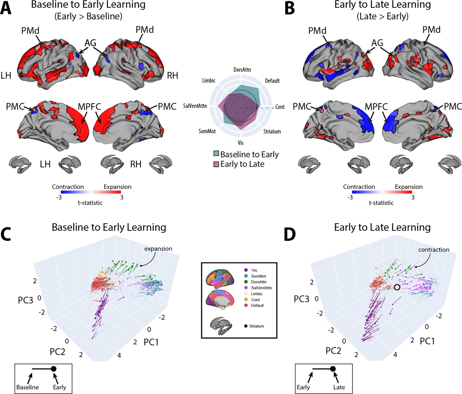
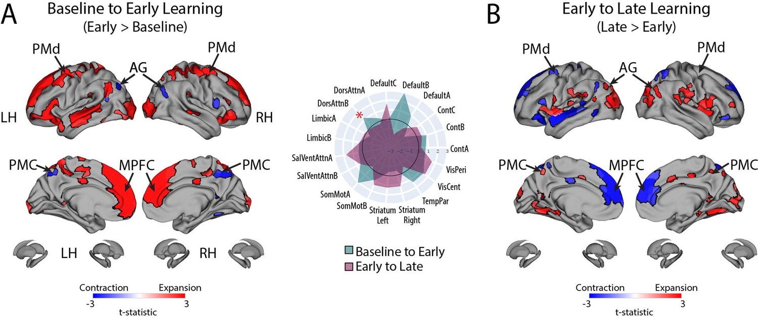
Changes in manifold structure during reward-based motor learning.
(A, B) Pairwise contrasts of eccentricity between task epochs (N=36). Positive (red) and negative (blue) values show significant increases and decreases in eccentricity (i.e., expansion and contraction along the manifold), respectively, following false discovery rate (FDR) correction for region-wise paired t-tests (at q < 0.05). The spider plot, at center, summarizes these patterns of changes in connectivity at the network-level (according to the Yeo networks, Thomas Yeo et al., 2011). Note that the black circle in the spider plot denotes t = 0 (i.e., no change in eccentricity between the epochs being compared). Radial axis values indicate t-values for the associated contrast (see color legend). (C, D) Temporal trajectories of statistically significant regions from (A) and (B), shown in the low-dimensional manifold space. Traces show the displacement of each region for the relevant contrast and filled colored circles indicate each region’s final position along the manifold for a given contrast (see insets for legends). Each region is colored according to its functional network assignment (middle). Nonsignificant regions are denoted by the gray point cloud. White circle with black bordering denotes the center of the manifold (manifold centroid).
Figure 4—figure supplement 1
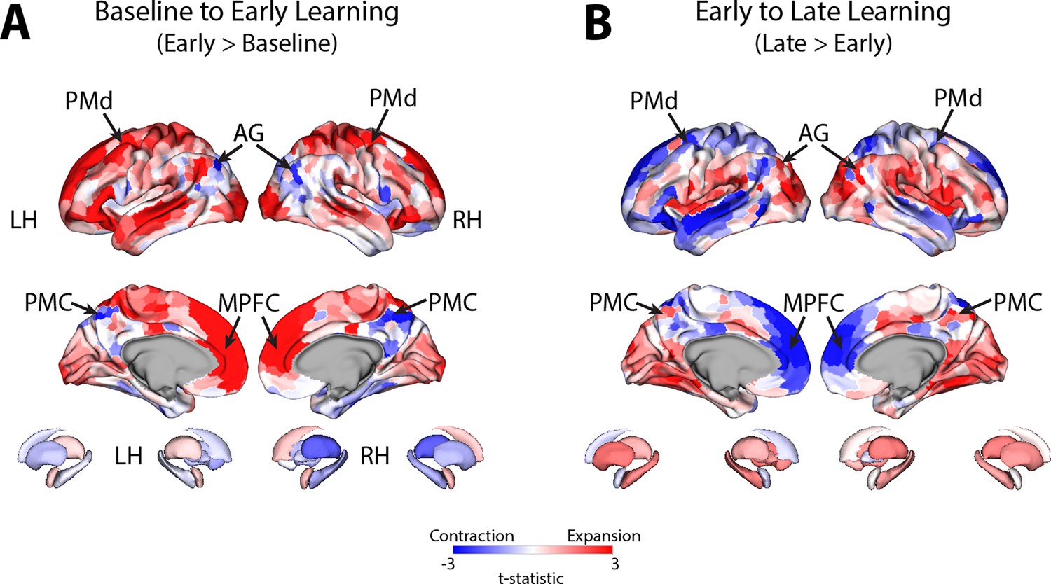
Unthresholded maps of changes in manifold structure during early and late learning.
(A, B) Pairwise contrasts of eccentricity between task epochs (N=36). Positive (red) and negative (blue) values denote increases and decreases in eccentricity (i.e., expansion and contraction along the manifold), respectively. The data shown in this figure is an unthresholded version of the data shown in Figure 4.
Figure 4—figure supplement 2
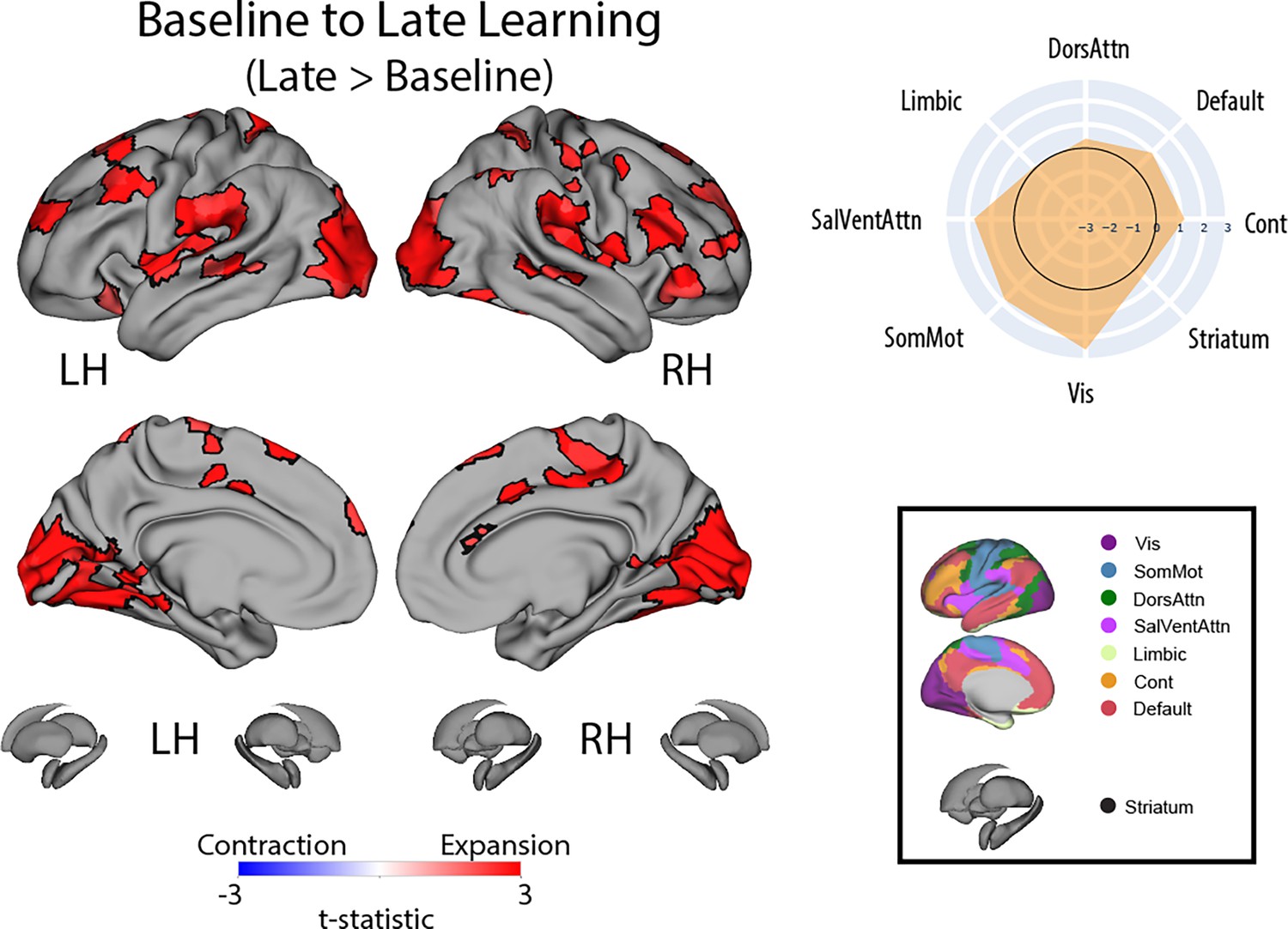
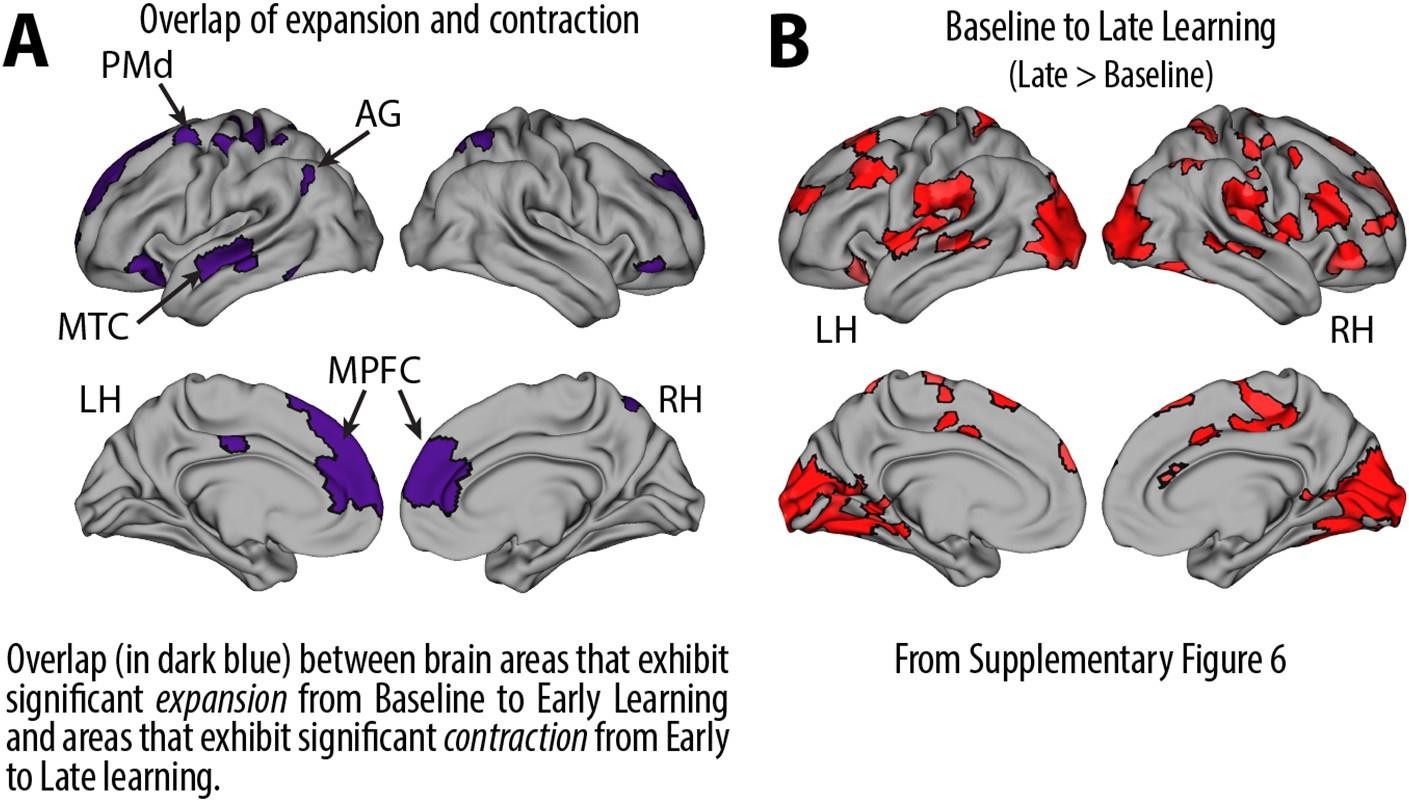
Changes in manifold structure from baseline to late learning.
Positive (red) and negative (blue) values show significant increases and decreases in eccentricity (i.e., expansion and contraction along the manifold), respectively, following false discovery rate (FDR) correction for region-wise paired t-tests (at q < 0.05; N=36). The spider plot, at the right, summarizes these patterns of changes in connectivity at the network-level (according to the Yeo networks). Note that the black circle in the spider plot denotes t = 0 (i.e., no change in eccentricity between the epochs being compared). Radial axis values indicate t-values for the associated contrast.
Figure 4—figure supplement 3
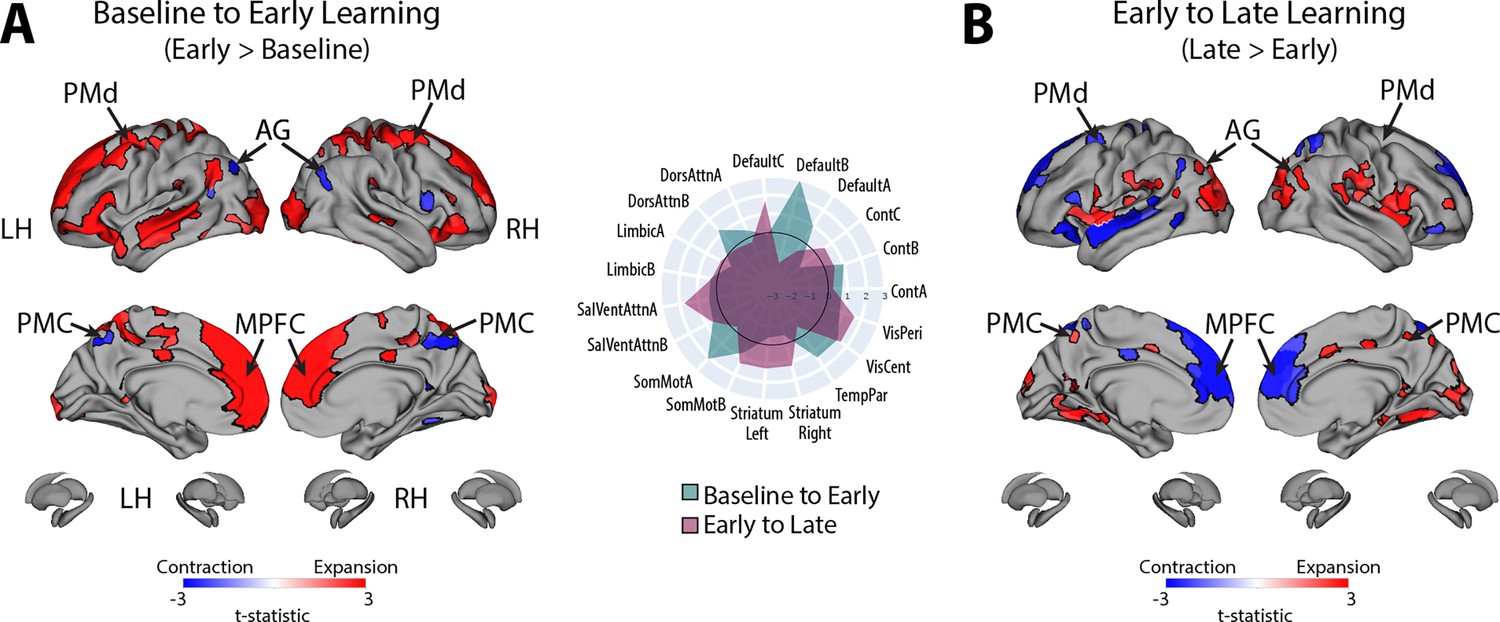
Changes in manifold structure during reward-based motor learning for the Yeo 17 network parcellation.
(A, B) Pairwise contrasts of eccentricity between task epochs (N=36). Positive (red) and negative (blue) values show significant increases and decreases in eccentricity (i.e., expansion and contraction along the manifold), respectively, following false discovery rate (FDR) correction for region-wise paired t-tests (at q < 0.05). This data is the same as shown in Figure 4. However, the spider plot, at center, summarizes these patterns of changes in connectivity at the 17-network-level (according to the Yeo networks, Thomas Yeo et al., 2011). Note that the black circle in the spider plot denotes t = 0 (i.e., no change in eccentricity between the epochs being compared). Radial axis values indicate t-values for the associated contrast (see color legend).
Figure 5 with 1 supplement
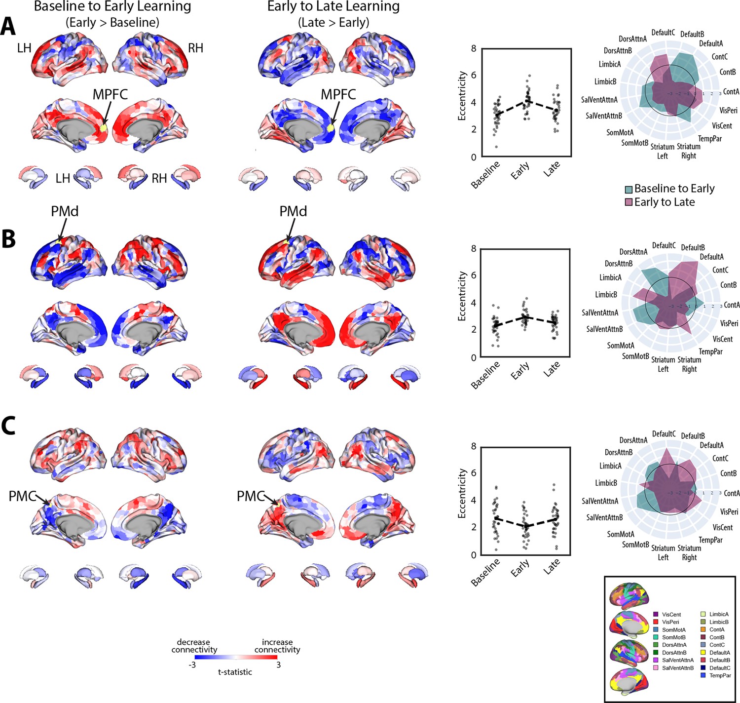
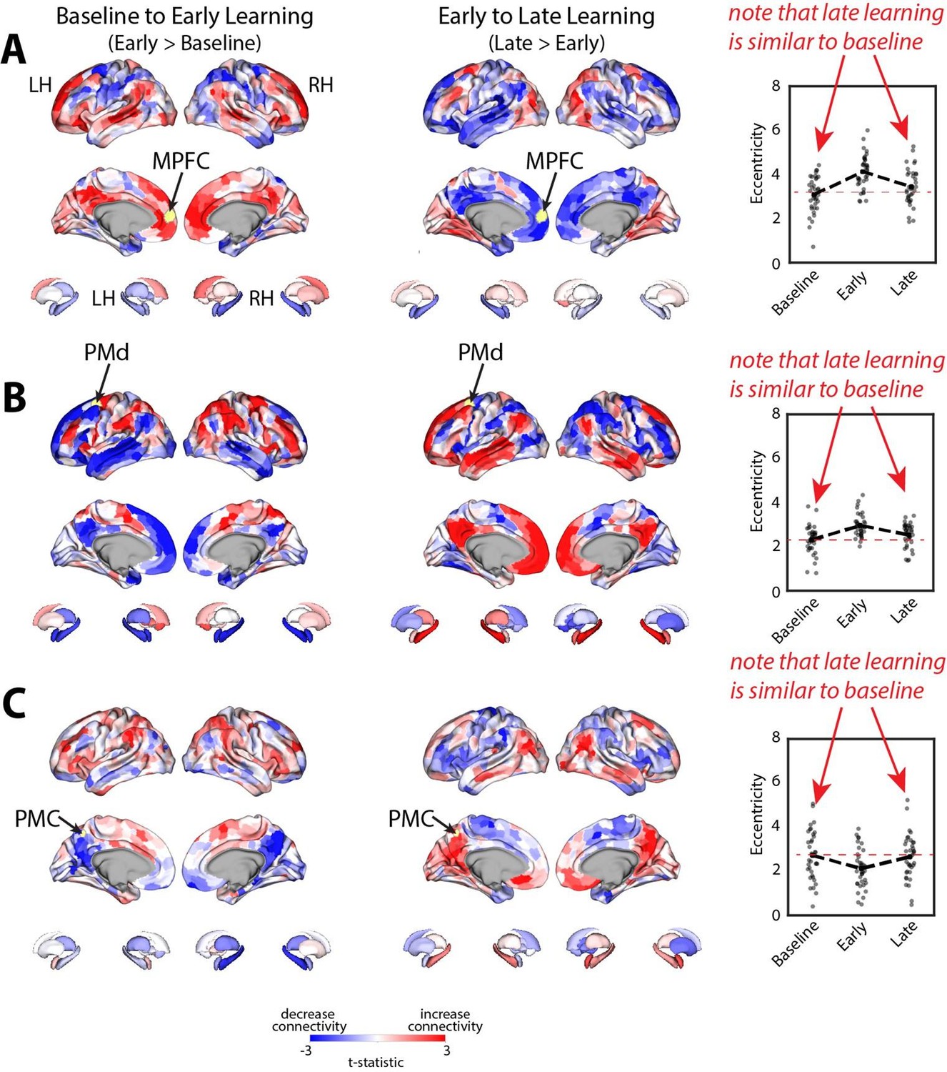
Main patterns of connectivity changes that underlie manifold expansions and contractions.
(A–C) Connectivity changes for each seed region. Selected seed regions are shown in yellow and are also indicated by arrows. Positive (red) and negative (blue) values show increases and decreases in connectivity, respectively, from baseline to early learning (leftmost panel) and early to late learning (second from leftmost panel). Second from the rightmost panel shows the eccentricity of each region for each participant (N=36), with the black dashed line showing the group mean for each task epoch. Rightmost panel contains spider plots, which summarize these patterns of changes in connectivity at the network level (according to the Yeo 17-networks parcellation; Thomas Yeo et al., 2011). Note that the black circle in the spider plot denotes t = 0 (i.e., zero change in eccentricity between the epochs being compared). Radial axis values indicate t-values for associated contrast (see color legend).
Figure 5—figure supplement 1
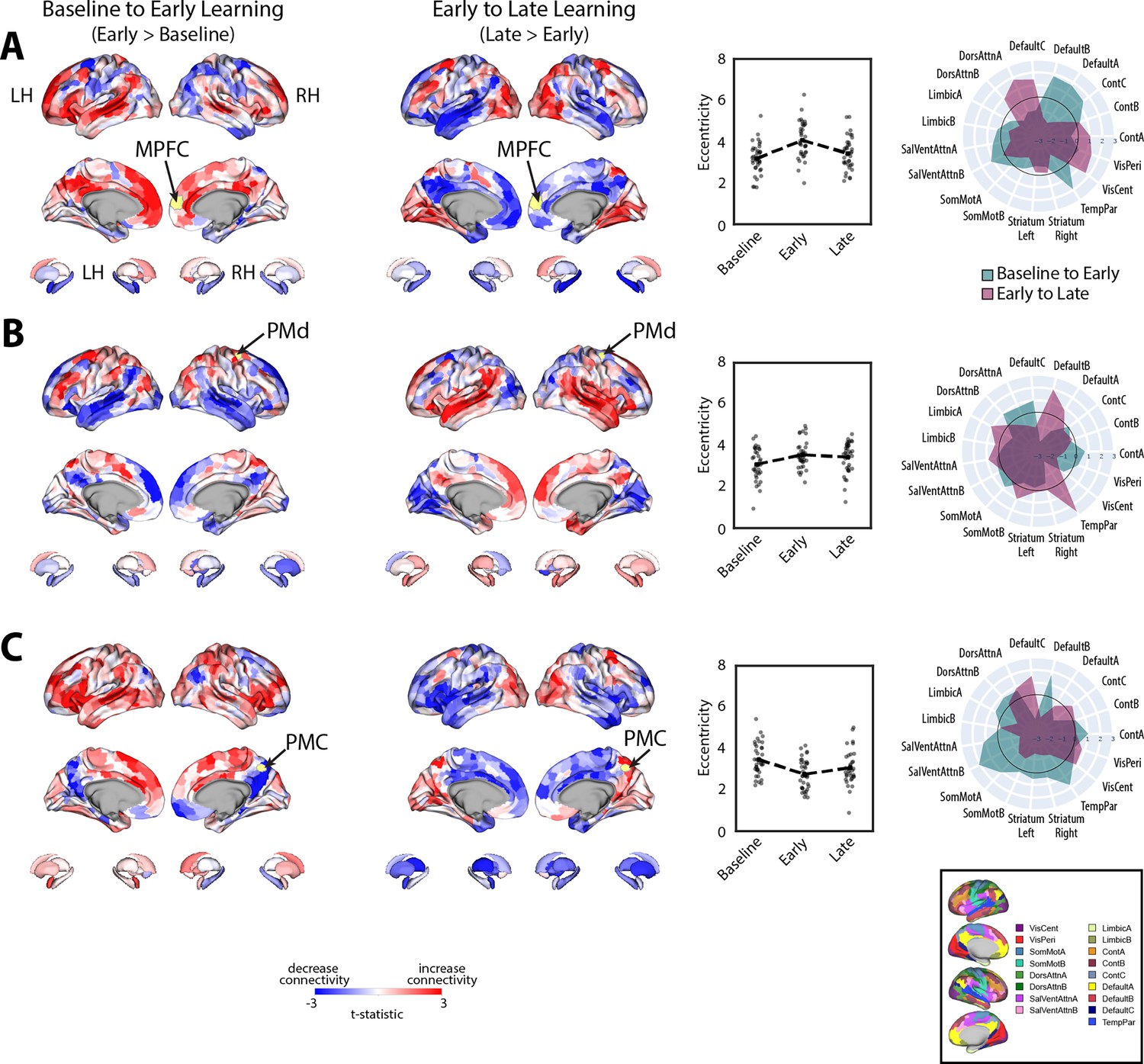
Patterns of connectivity changes that underlie manifold expansions and contractions for right-hemisphere regions.
(A–C) Connectivity changes for each seed region. Selected seed regions are shown in yellow and are also indicated by arrows. Positive (red) and negative (blue) values show increases and decreases in connectivity, respectively, from baseline to early learning (leftmost panel) and early to late learning (second from leftmost panel). Second from the rightmost panel shows the eccentricity of each region for each participant (N=36), with the black dashed line plot overlay showing the group mean for each task epoch. Rightmost panel contains spider plots, which summarize these patterns of changes in connectivity at the network level (according to the Yeo 17-networks parcellation; Thomas Yeo et al., 2011). Note that the black circle in the spider plot denotes t = 0 (i.e., zero change in eccentricity between the epochs being compared). Radial axis values indicate t-values for associated contrast.
Figure 6
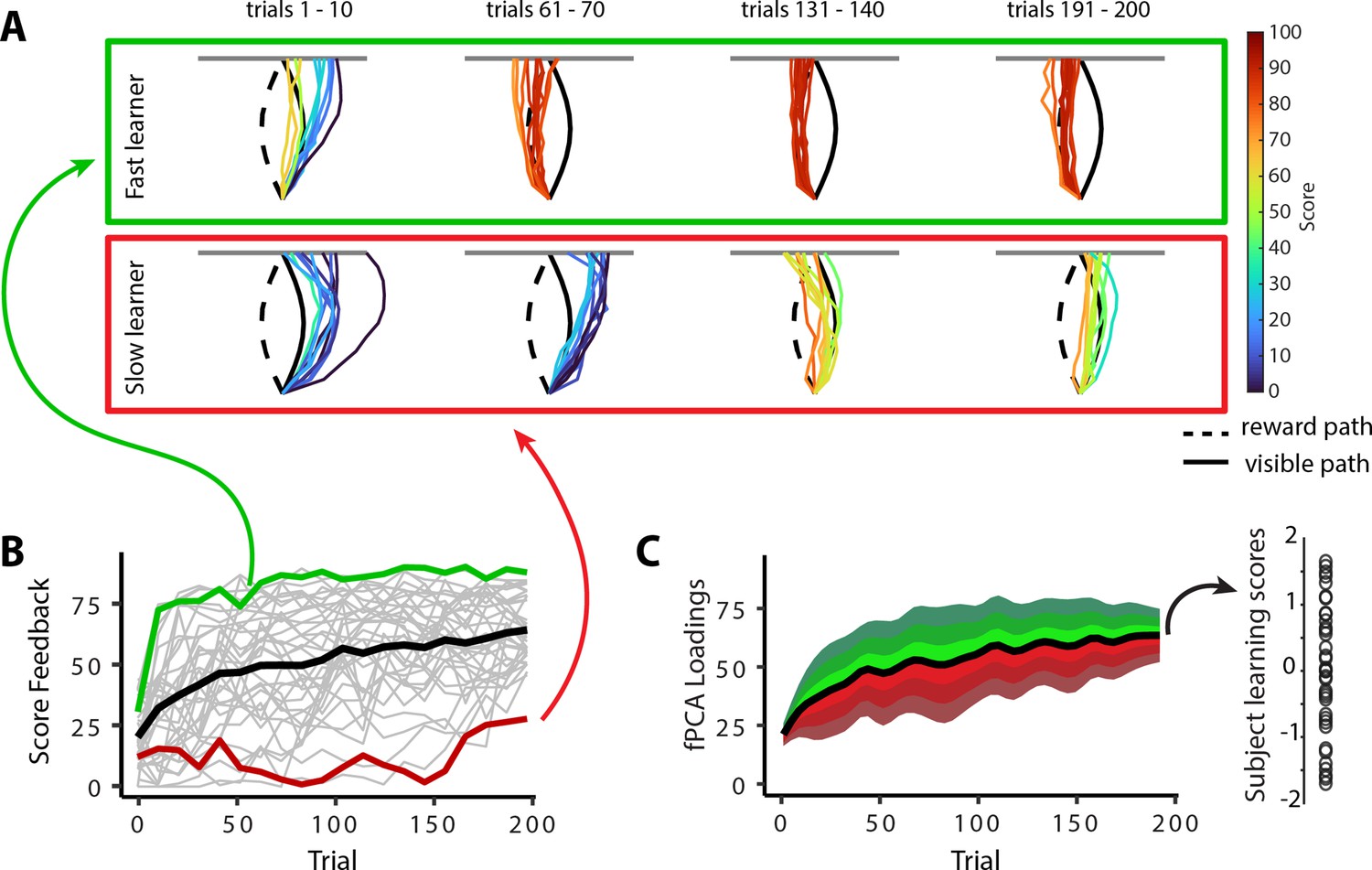
Individual differences in subject learning performance.
(A) Examples of a good learner (bordered in green) and poor learner (bordered in red). (B) Individual subject learning curves for the task. Solid black line denotes the mean across all subjects (N=36), whereas light gray lines denote individual participants. The green and red traces denote the learning curves for the example good and poor learners denoted in (A). (C) Derivation of subject learning scores. We performed functional principal component analysis (fPCA) on subjects’ learning curves in order to identify the dominant patterns of variability during learning. The top component, which encodes overall learning, explained the majority of the observed variance (~75%). The green and red bands denote the effect of positive and negative component scores, respectively, relative to mean performance. Thus, subjects who learned more quickly than average have a higher loading (in green) on this ‘learning score’ component than subjects who learned more slowly (in red) than average. The plot at the right denotes the loading for each participant (open circles) onto this learning score component.
Figure 7
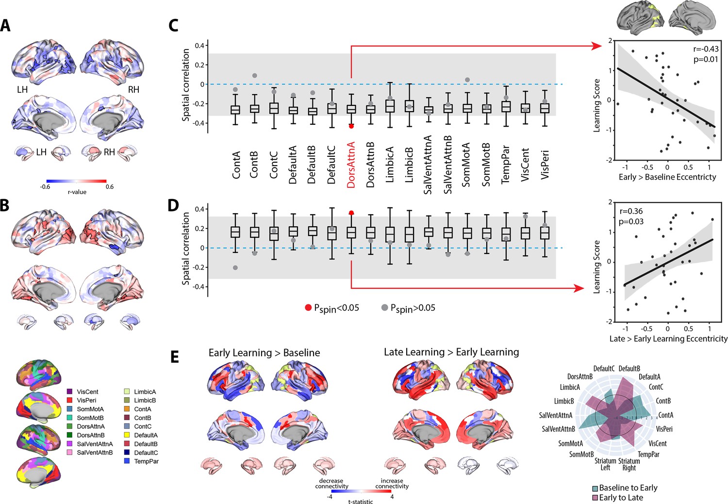
Relationship between learning performance and regional changes in eccentricity.
(A, B) Whole-brain correlation map between subject learning score and the change in regional eccentricity from baseline to early learning (A) and early to late learning (B). Black bordering denotes regions that are significant at p<0.05. (C, D) Results of the spin-test permutation procedure, assessing whether the topography of correlations in (A) and (B) are specific to individual functional brain networks. Single points indicate the real correlation value for each of the 17 Yeo et al. networks (Thomas Yeo et al., 2011), whereas the boxplots represent the parameters of a null distribution of correlations derived from 1000 iterations of a spatial autocorrelation-preserving null model (Markello et al., 2022; Váša et al., 2018). In the boxplots, the ends of the boxes represent the first (25%) and third (75%) quartiles, the center line represents the median, and the whiskers represent the min-max range of the null distribution. All correlations were corrected for multiple comparisons (q < 0.05). The dashed horizontal blue line indicates a correlation value of zero and the gray shading encompasses correlation values that do not significantly differ from zero (p>0.05). (Note that in the spin-test procedure, due to the sign of the correlations, it is possible for some networks to be significantly different from the null distribution, and yet not significantly different from zero. Thus, to be considered significant in our analyses, a brain network was required to satisfy both constraints; i.e., show a correlation that is significantly different from zero and from the spatial null distribution.) Right, scatterplots show the relationships between subject learning score and the change in eccentricity from baseline to early learning (top) and early to late learning (bottom) for the DAN-A network (depicted in yellow on the cortical surface at top), the only brain network to satisfy the two constraints of our statistical testing procedure. Black line denotes the best-fit regression line, with shading indicating ±1 SEM. Dots indicate single participants (N=36). (E) Connectivity changes for the DAN-A network (highlighted in yellow) across epochs. Positive (red) and negative (blue) values show increases and decreases in connectivity, respectively, from baseline to early learning (left panel) and early to late learning (right panel). Spider plot, at the right, summarizes the patterns of changes in connectivity at the network-level. Note that the black circle in the spider plot denotes t = 0 (i.e., no change in eccentricity between the epochs being compared). Radial axis values indicate t-values for associated contrast (see color legend). VisCent: visual central; VisPer: visual peripheral; SomMotA: somatomotor A; SomMotB: somatomotor B; TempPar: temporal parietal; DorsAttnA: dorsal attention A; DorsAttnB: dorsal attention B; SalVentAttnA: salience/ventral attention A; SalVentAttnB: salience/ventral attention B; ContA: control A; ContB: control B; ContC: control C.
Author response image 1
Author response image 2
Author response image 3

Behavioral measures of learning across the task.
(A-D) shows average participant reward scores (A), reaction times (B), movement times (C) and path variability (D) over the course of the task. In each plot, the black line denotes the mean across participants and the gray banding denotes +/- 1 SEM. The three equal-length task epochs for subsequent neural analyses are indicated by the gray shaded boxes.
Author response image 4

Individual differences in subject learning performance.
(A) Examples of a good learner (bordered in green) and poor learner (bordered in red). (B) Individual subject learning curves for the task. Solid black line denotes the mean across all subjects whereas light gray lines denote individual participants. The green and red traces denote the learning curves for the example good and poor learners denoted in A. (C) Derivation of subject learning scores. We performed functional principal component analysis (fPCA) on subjects’ learning curves in order to identify the dominant patterns of variability during learning. The top component, which encodes overall learning, explained the majority of the observed variance (~75%). The green and red bands denote the effect of positive and negative component scores, respectively, relative to mean performance. Thus, subjects who learned more quickly than average have a higher loading (in green) on this ‘Learning score’ component than subjects who learned more slowly (in red) than average. The plot at right denotes the loading for each participant (open circles) onto this Learning score component.
Author response image 5

Variability in learning across subjects.
Plots show representative trajectory data from each subject (n=36) over the course of the 200 learning trials. Coloured traces show individual trials over time (each trace is separated by ten trials, e.g., trial 1, 10, 20, 30, etc.) to give a sense of the trajectory changes throughout the task (20 trials in total are shown for each subject).
Author response image 6

Author response image 7
Author response image 8
Author response image 9

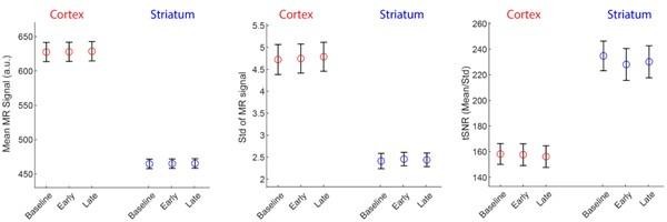
Examination of overall changes in activity across regions.
(A) Mean z-score maps across subjects for the Baseline (top), Early Learning (middle) and Late learning (bottom) epochs. (B) Mean z-score across brain regions for each epoch. Error bars represent +/- 1 SEM. (C) Pairwise contrasts of the z-score signal between task epochs. Positive (red) and negative (blue) values show significant increases and decreases in z-score signal, respectively, following FDR correction for region-wise paired t-tests (at q<0.05).
Additional files
Download links
A two-part list of links to download the article, or parts of the article, in various formats.
Downloads (link to download the article as PDF)
Open citations (links to open the citations from this article in various online reference manager services)
Cite this article (links to download the citations from this article in formats compatible with various reference manager tools)
Reconfigurations of cortical manifold structure during reward-based motor learning
eLife 12:RP91928.
https://doi.org/10.7554/eLife.91928.3


