osl-dynamics, a toolbox for modeling fast dynamic brain activity
- Oxford Centre for Human Brain Activity, Wellcome Centre for Integrative Neuroimaging, Department of Psychiatry, University of Oxford, United Kingdom
- Centre for Human Brain Health, School of Psychology, University of Birmingham, United Kingdom
- Center for Functionally Integrative Neuroscience, Department of Clinical Medicine, Aarhus University, Denmark
Figures
Figure 1 with 1 supplement
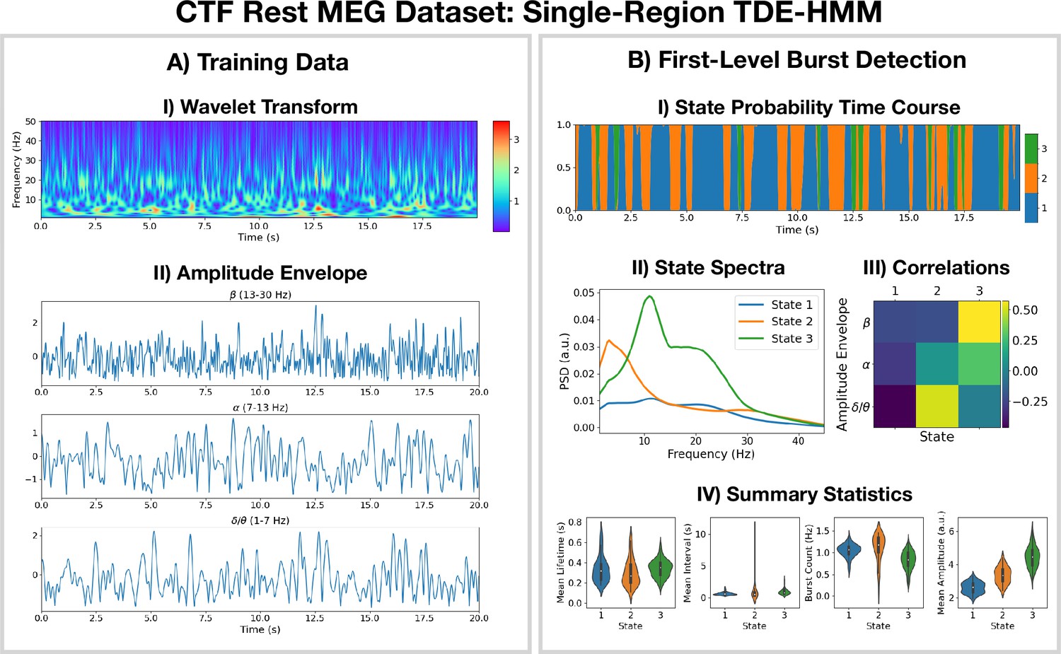
Burst detection: single region source reconstructed magnetoencephalography (MEG) data (left motor cortex) shows short-lived bursts of oscillatory activity.
(A.I) Dynamic spectral properties of the first 20 s of the time series from the first subject. (A.II) Amplitude envelope calculated after bandpass filtering the time series over the -band (top), -band (middle), and -band (bottom). (B.I) The inferred state probability time course for the first 20 s of the first subject. (B.II) The power spectral density (PSD) of each state. (B.III) Pearson correlation of each state probability time course with the amplitude envelopes for different frequency bands. (B.IV) Distribution over subjects for summary statistics characterizing the bursts. Note that no additional bandpass filtering was done to the source data when calculating the mean amplitude. The script used to generate the results in this figure is here: https://github.com/OHBA-analysis/osl-dynamics/blob/main/examples/toolbox_paper/ctf_rest/tde_hmm_bursts.py; (Gohil, 2024).
Figure 1—figure supplement 1
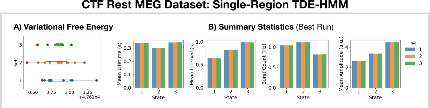
Reproducibility of the CTF rest magnetoencephalography (MEG) dataset single-region TDE-HMM analysis.
(A) Variational free energy for three sets of 10 runs. (B) Summary statistics for the best run from each set (indicated by the red dot in A).
Figure 2 with 1 supplement
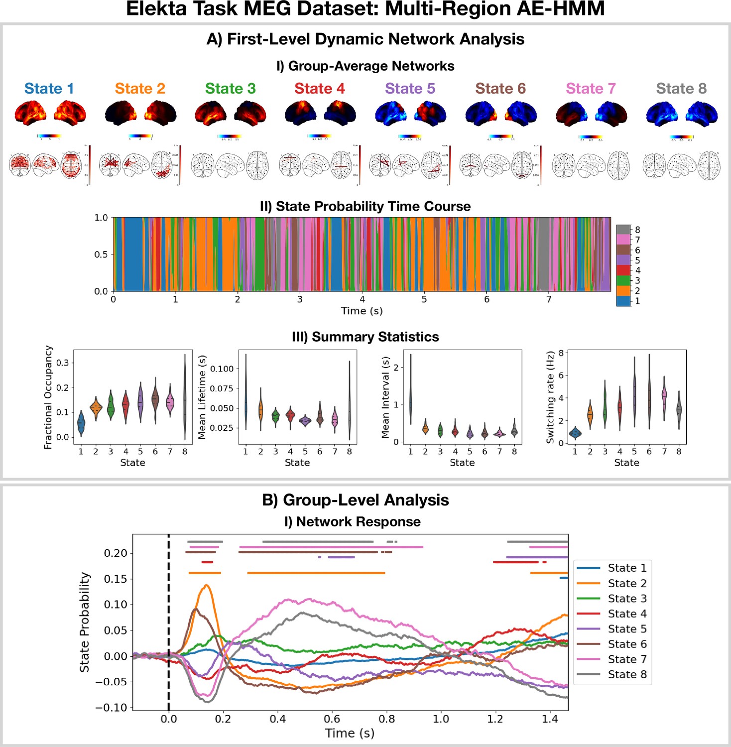
Dynamic network detection: a multi-region AE-HMM trained on the Elekta task magnetoencephalography (MEG) dataset reveals functional networks with fast dynamics that are related to the task.
(A.I) For each state, group-averaged amplitude maps relative to the mean across states (top) and absolute amplitude envelope correlation networks (bottom). (A.II) State probability time course for the first 8 s of the first subject. (A.III) Distribution over subjects for the summary statistics for each state. (B.I) State time courses (Viterbi path) epoched around the presentation of visual stimuli. The horizontal bars indicate time points with p<0.05. The maximum statistic pooling over states and time points was used in permutation testing to control for the family-wise error rate. The script used to generate the results in this figure is here: https://github.com/OHBA-analysis/osl-dynamics/blob/main/examples/toolbox_paper/elekta_task/ae_hmm.py.
Figure 2—figure supplement 1
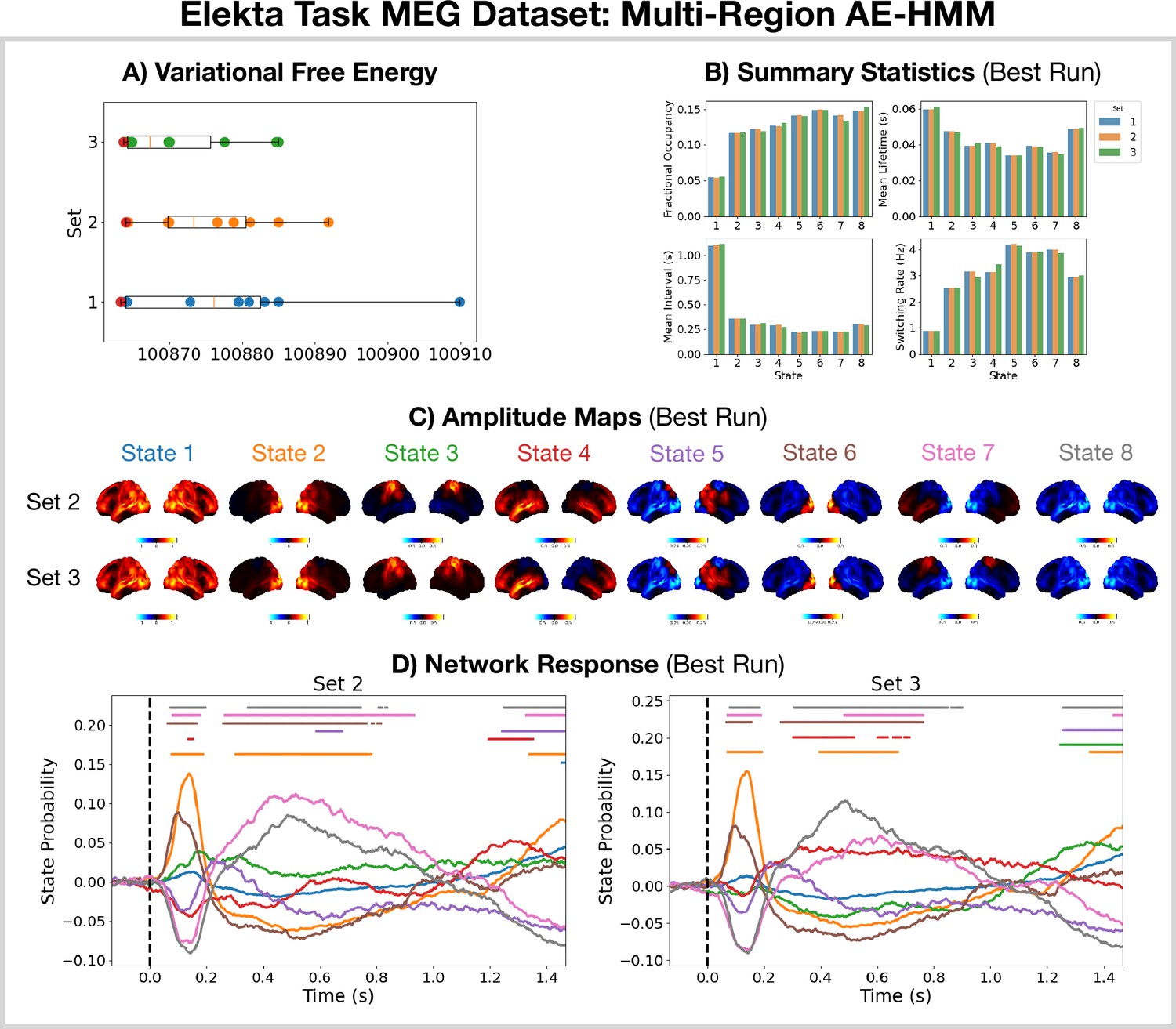
Reproducibility of the Elekta task magnetoencephalography (MEG) dataset multi-region AE-HMM analysis.
(A) Variational free energy for three sets of 10 runs. (B) Summary statistics for the best run from each set (indicated by the red dot in A). (C) Amplitude maps relative to the mean across states for the best run from sets 2 and 3. (D) Network response to the visual task for sets 2 and 3. The horizontal bars indicate time points with p<0.05. The maximum statistic pooling over states and time was used in permutation testing to control for the family-wise error rate.
Figure 3 with 1 supplement
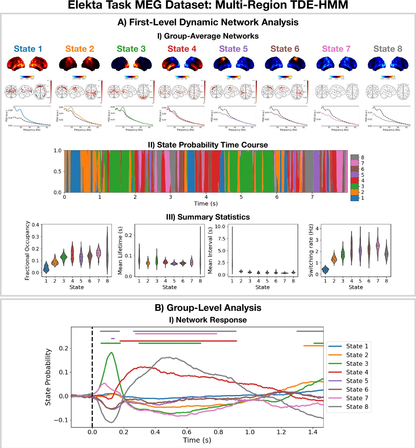
Dynamic network detection: a multi-region TDE-HMM trained on the Elekta task magnetoencephalography (MEG) dataset reveals spectrally distinct functional networks with fast dynamics.
(A.I) For each state, group-averaged power maps relative to the mean across states (top), coherence networks (middle), and power spectral density (PSD) averaged over regions (bottom), both the state-specific (colored solid line), and static PSD (i.e. the average across states, dashed black line) are shown. (A.II) State probability time course for the first 8 s of the first subject. (A.III) Distribution over subjects for the summary statistics for each state. (B.I) State time courses (Viterbi path) epoched around the presentation of visual stimuli. The horizontal bars indicate time points with p<0.05. The maximum statistic pooling over states and time points was used in permutation testing to control for the family-wise error rate. The script used to generate the results in this figure is here: https://github.com/OHBA-analysis/osl-dynamics/blob/main/examples/toolbox_paper/elekta_task/tde_hmm.py.
Figure 3—figure supplement 1
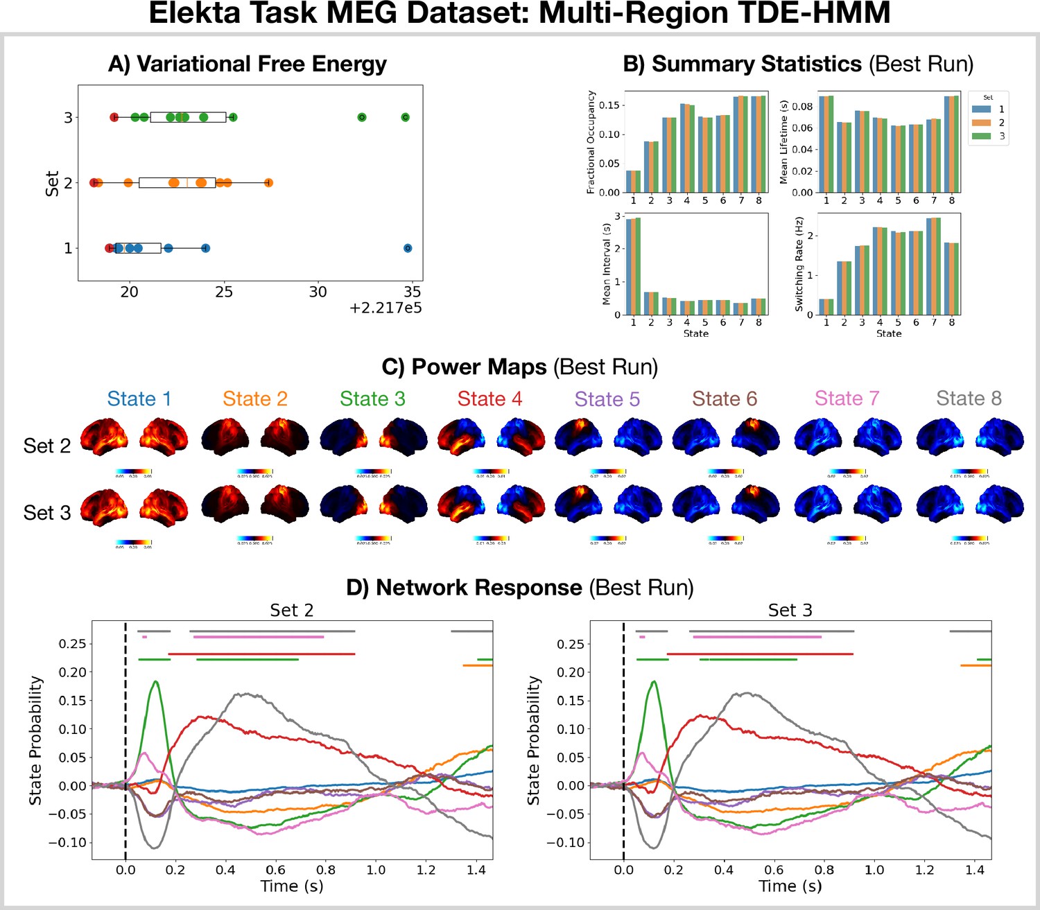
Reproducibility of the Elekta task magnetoencephalography (MEG) dataset multi-region TDE-HMM analysis.
(A) Variational free energy for three sets of 10 runs. (B) Summary statistics for the best run from each set (indicated by the red dot in A). (C) Power maps relative to the mean across states for the best run from sets 2 and 3. (D) Network response to the visual task for sets 2 and 3. The horizontal bars indicate time points with p<0.05. The maximum statistic pooling over states and time was used in permutation testing to control for the family-wise error rate.
Figure 4 with 1 supplement
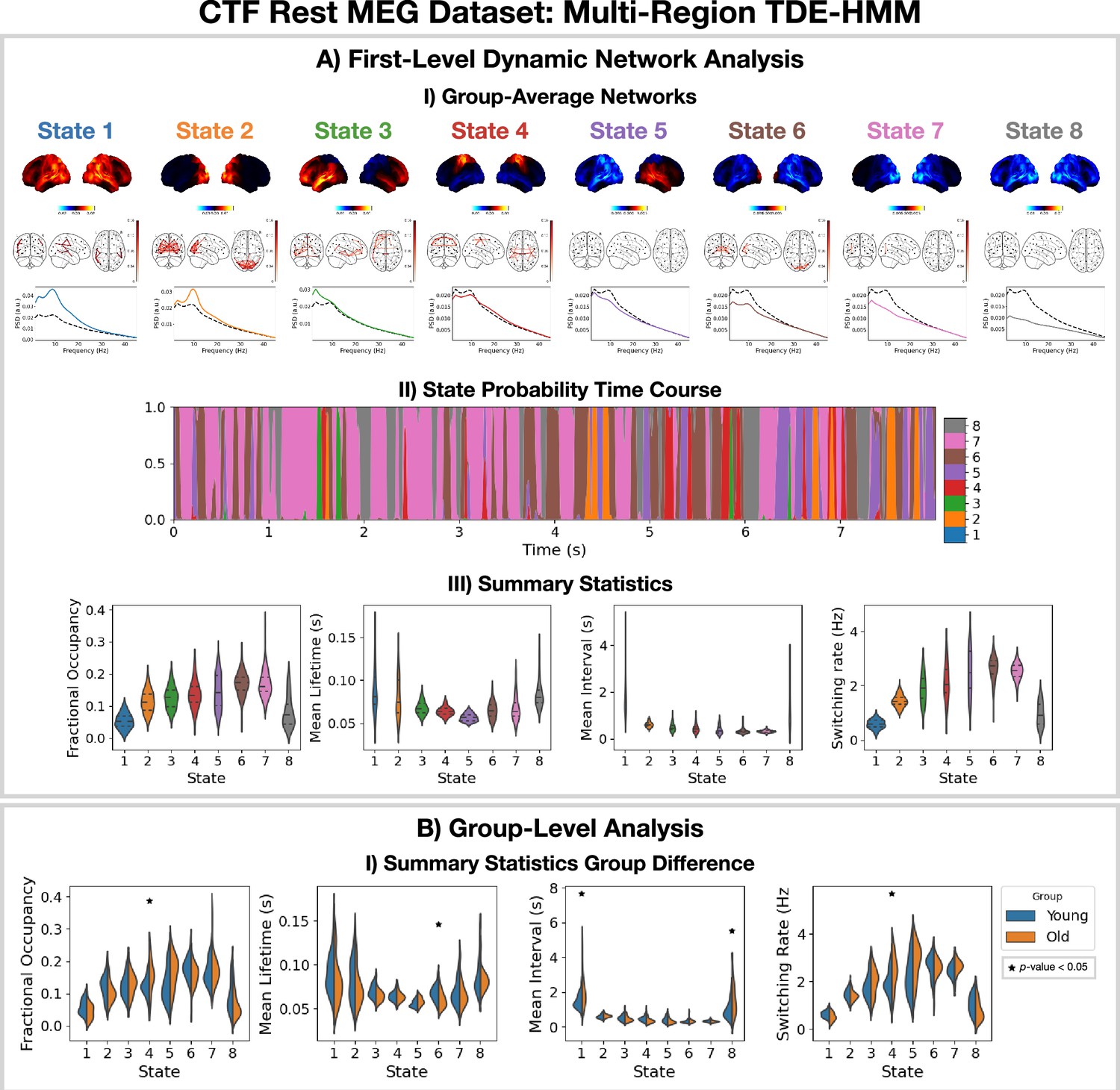
Dynamic network detection: a multi-region TDE-HMM trained on the CTF rest magnetoencephalography (MEG) dataset identifies the same functional networks to those found with the Elekta task MEG dataset and reveals differences in the dynamics for young vs old groups.
(A.I) For each state, group-averaged power maps relative to mean across states (top), absolute coherence networks (middle) and power spectral density (PSD) averaged over regions (bottom), both the state-specific (colored solid line) and static PSD (i.e. the average across states, dashed black line) are shown. (A.II) State probability time course for the first 8 s of the first subject and run. (A.III) Distribution over subjects for the summary statistics of each state. (B.I) Comparison of the summary statistics for a young (18–34 years old) and old (34–60 years old) group. The star indicates a p<0.05. The maximum statistic pooling over states and metrics was used in permutation testing to control for the family-wise error rate. The script used to generate the results in this figure is here: https://github.com/OHBA-analysis/osl-dynamics/blob/main/examples/toolbox_paper/ctf_rest/tde_hmm_networks.py; (Gohil, 2024).
Figure 4—figure supplement 1
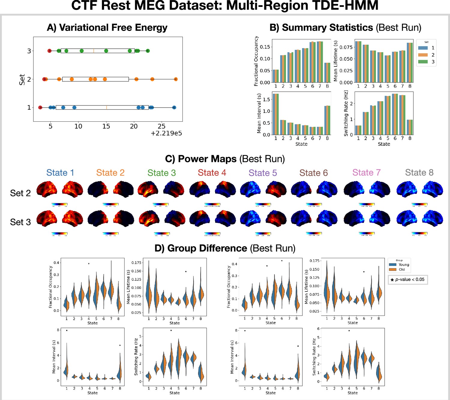
Reproducibility of the CTF rest magnetoencephalography (MEG) dataset multi-region TDE-HMM analysis.
(A) Variational free energy for three sets of 10 runs. (B) Summary statistics for the best run from each set (indicated by the red dot in A). (C) Power maps relative to the mean across states for the best run from sets 2 and 3. (D) Comparison of the summary statistics for a young (18–34 years old) and old (34–60 years old) group. The star indicates a p<0.05. The maximum statistic pooling over states and metrics was used to control for the family-wise error rate.
Figure 5 with 1 supplement
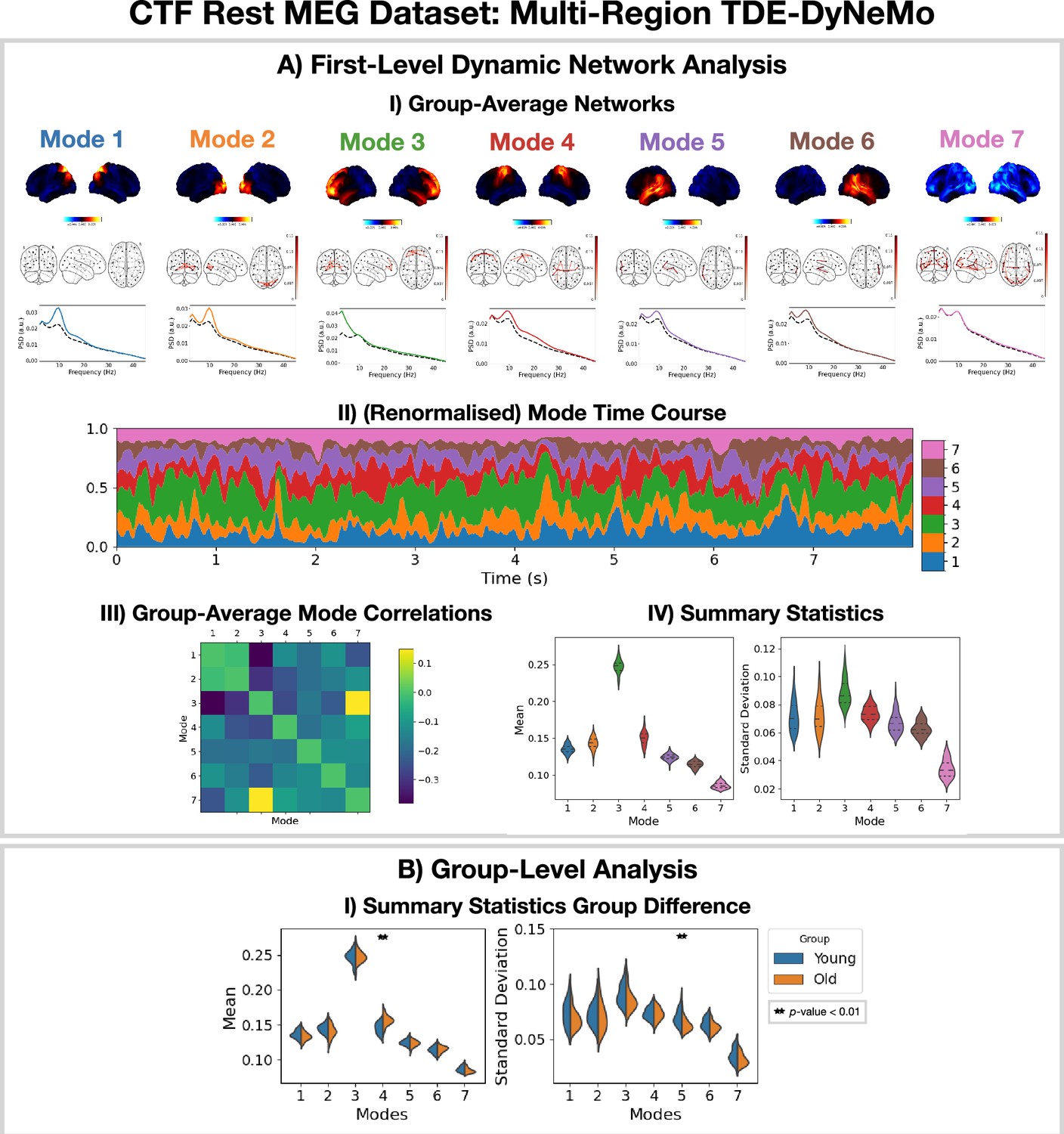
Dynamic network detection: a multi-region TDE-DyNeMo trained on the CTF rest magnetoencephalography (MEG) dataset reveals spectrally distinct modes that are more localized than Hidden Markov Model (HMM) states and overlap in time.
(A.I) For each mode, group-averaged power maps relative to the mean across modes (top), absolute coherence networks (middle), and power spectral density (PSD) averaged over regions (bottom), both the mode-specific (colored solid line) and static PSD (i.e. the average across modes, dashed black line) are shown. (A.II) Mode time course (mixing coefficients) renormalized using the trace of the mode covariances. (A.III) Pearson correlation between renormalized mode time courses calculated by concatenating the time series from each subject. (A.IV) Distribution over subjects for summary statistics (mean and standard deviation) of the renormalized mode time courses. (B.I) Comparison of the summary statistics for a young (18–34 years old) and old (34–60 years old) group. The maximum statistic pooling over modes and metrics was used in permutation testing to control for the family-wise error rate. The script used to generate the results in this figure is here: https://github.com/OHBA-analysis/osl-dynamics/blob/main/examples/toolbox_paper/ctf_rest/tde_dynemo_networks.py.
Figure 5—figure supplement 1
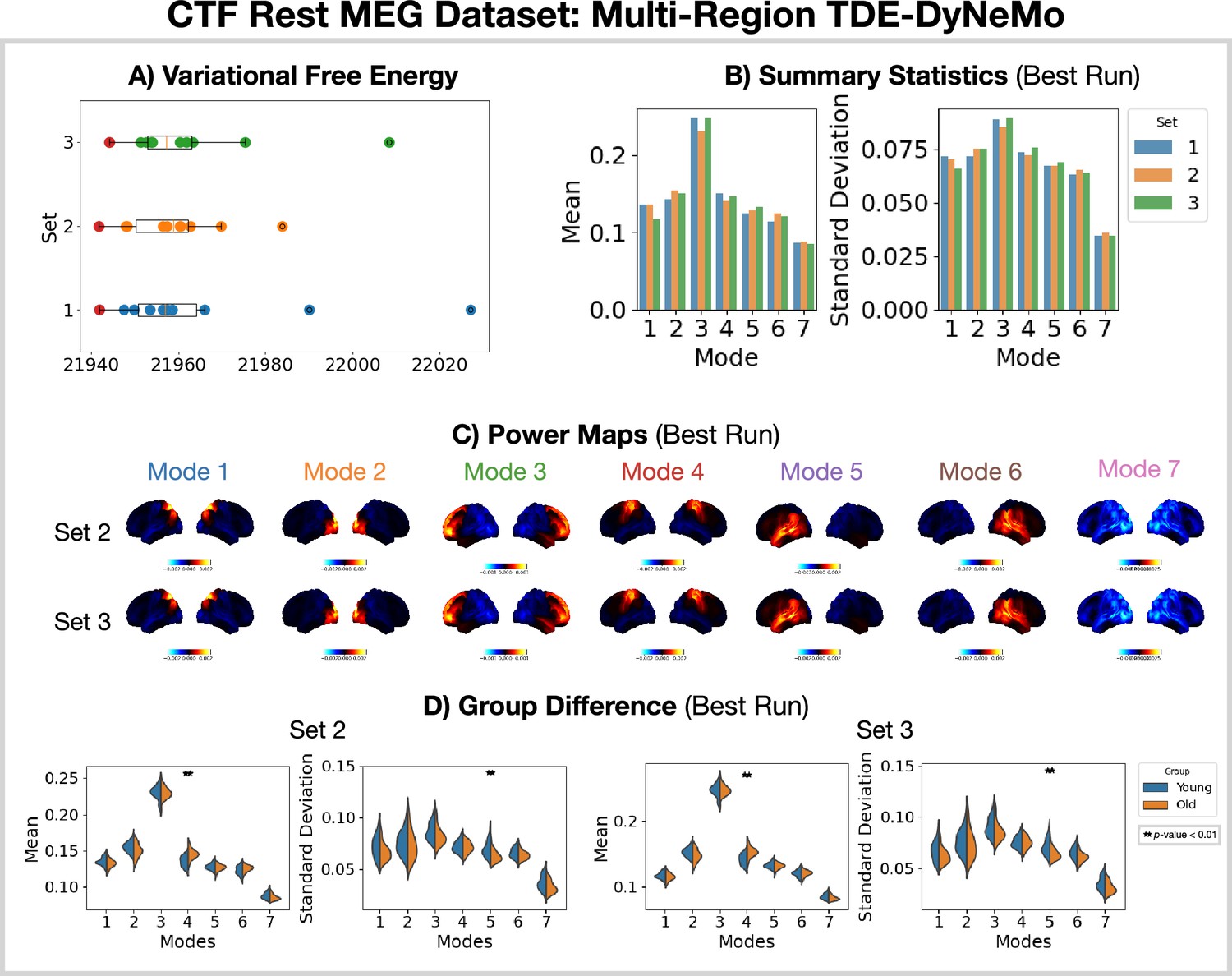
Reproducibility of the CTF rest magnetoencephalography (MEG) dataset multi-region TDE-DyNeMo analysis.
(A) Variational free energy for three sets of 10 runs. (B) Summary statistics for the best run from each set (indicated by the red dot in A). (C) Power maps relative to the mean across modes for the best run from sets 2 and 3. (D) Comparison of the summary statistics for a young (18–34 years old) and old (34–60 years old) group. The double star indicates a p<0.01. The maximum statistic pooling over modes and metrics was used to control for the family-wise error rate.
Figure 6

Static network detection: osl-dynamics can also be used to perform static network analyses (including functional connectivity).
In the CTF rest magnetoencephalography (MEG) dataset, this reveals frequency-specific differences in the static functional networks of young (18–34 years old) and old (34–60 years old) participants. Group-average power spectral density (PSD) (averaged over subjects and parcels, (A.I) power maps (A.II) coherence networks (A.III) and AEC networks (A.IV) for the canonical frequency bands (). (B.I) Power difference for old minus young (top) and p-values (bottom). Only frequency bands with at least one parcel with a p<0.05 are shown, the rest are marked with n.s. (none significant). B.II) Amplitude envelope correlation (AEC) difference for old minus young only showing edges with a p<0.05. The maximum statistic pooling over frequency bands and parcels/edges was used in permutation testing to control for the family-wise error rate. The script used to generate the results in this figure is here: https://github.com/OHBA-analysis/osl-dynamics/blob/main/examples/toolbox_paper/ctf_rest/static_networks.py.
Figure 7
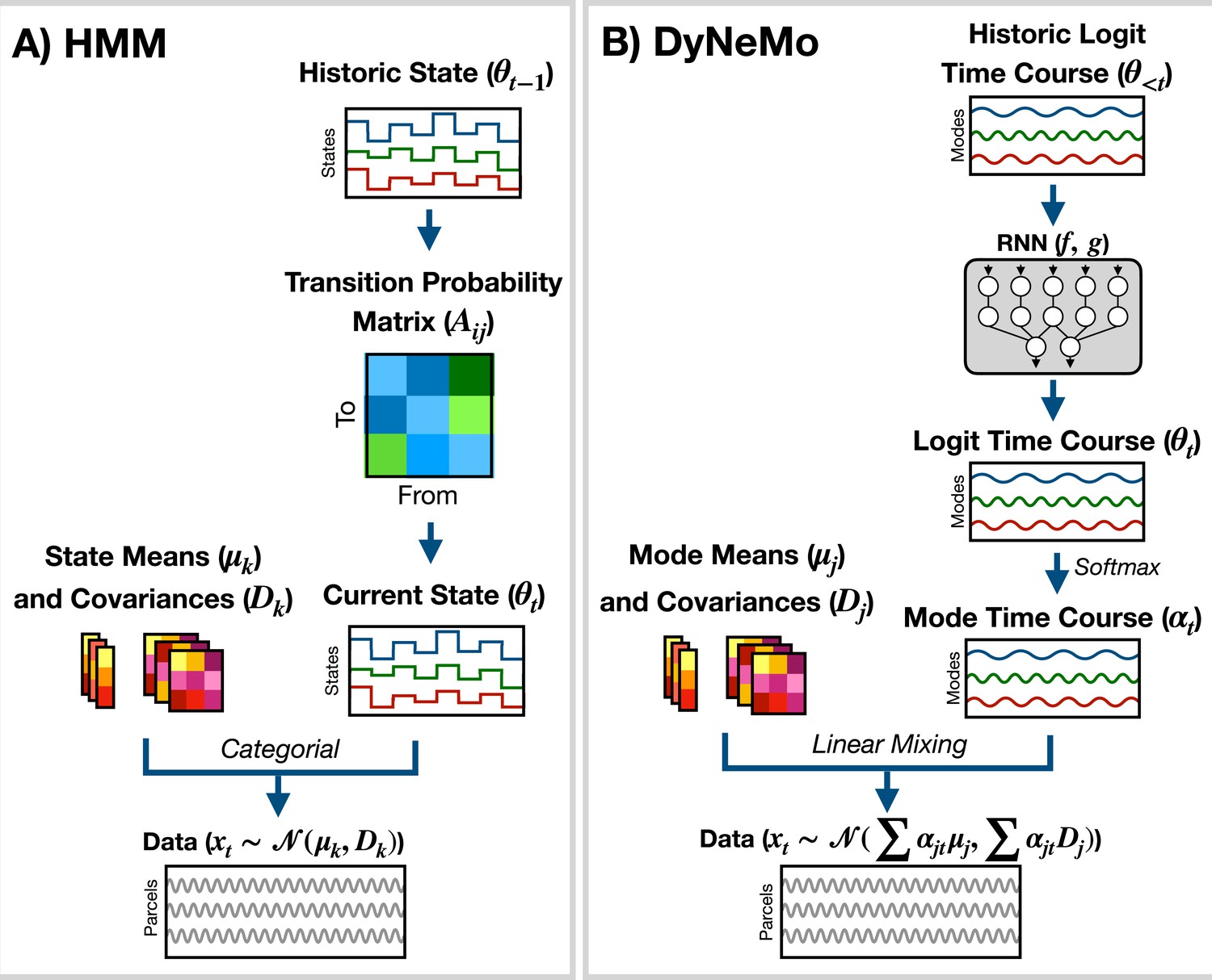
Generative models implemented in osl-dynamics.
(A) Hidden Markov Model (HMM) (Vidaurre et al., 2016; Vidaurre et al., 2018a). Here, data is generated using a hidden state () and observation model, which in our case is a multivariate normal distribution parameterized by a state mean () and covariance (). Only one state can be active at a given time point. Dynamics are modeled via state switching using a transition probability matrix (), which forecasts the probability of the current state based on the previous state. (B) Dynamic Network Modes (DyNeMo) (Gohil et al., 2022). Here, the data is generated using a linear combination of modes ( and ) and dynamics are modelled using a recurrent neural network (RNN: and ), which forecasts the probability of a particular mixing ratio () based on a long history of previous values via the underlying logits ().
Figure 8

Preprocessing and source reconstruction.
First, the sensor-level recordings are cleaned using standard signal processing techniques. This includes filtering, downsampling, and artifact removal. Following this, the sensor-level recordings are used to estimate source activity using a beamformer. Finally, we parcellate the data and perform corrections (orthogonalization and dipole sign flipping). Acronyms: electrocardiogram (ECG), electrooculogram (EOG), independent component analysis (ICA), linearly constrained minimum variance (LCMV). These steps can be performed with the OHBA Software Library: https://github.com/OHBA-analysis/osl, (copy archived at OHBA-analysis, 2024).
Figure 9
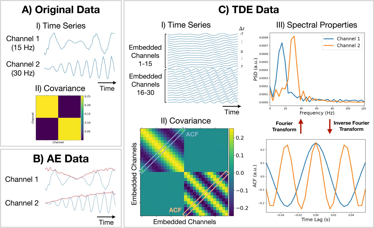
Methods for preparing training data.
(A.I) Original (simulated) time series data. Only a short segment (0.2 s) is shown. Channel 1 (2) is a modulated sine wave at 15 Hz (30 Hz) with noise added. (A.II) Covariance of the original data. (B) Amplitude envelope (AE) data (solid red line) and original data (dashed blue line). (C.I) Time-delay embedded (TDE) time series. An embedding window of ±7 lags was used. (C.II) Covariance of TDE data. (C.III) Spectral properties of the original data were estimated using the covariance matrix of TDE data. Acronyms: Autocorrelation function (ACF), Power spectral density (PSD).
Figure 10
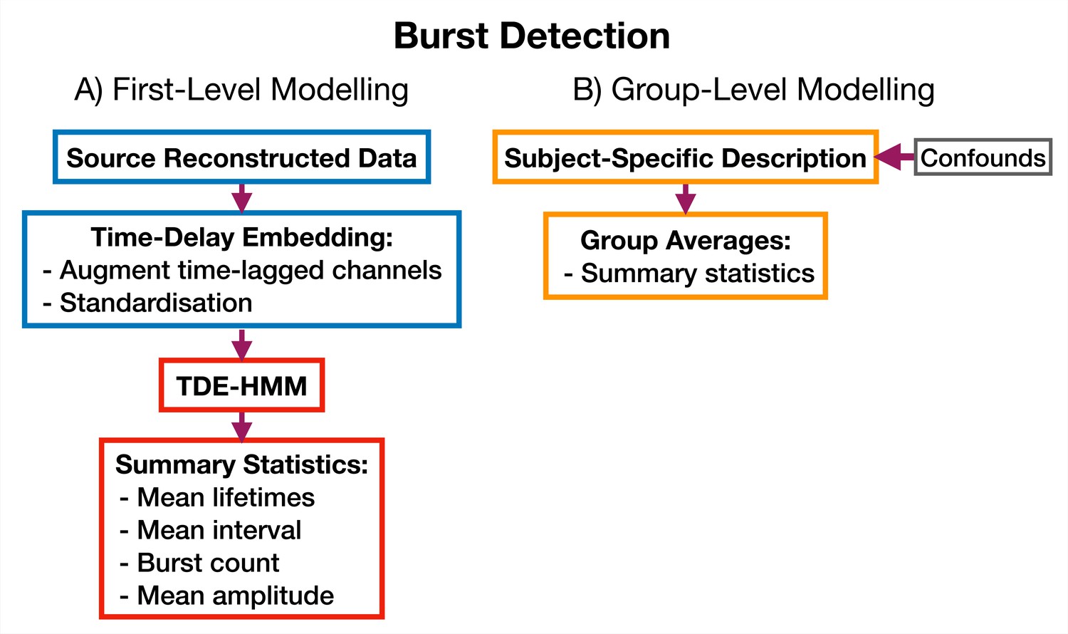
TDE-HMM burst detection pipeline.
This is run on a single region’s parcel time course. Separate Hidden Markov Models (HMMs) are trained for each region. (A) Source reconstructed data is prepared by performing time-delay embedding and standardization (z-transform). Following this an HMM is trained on the data and statistics that summarize the bursts are calculated from the inferred state time course. (B) Subject-specific metrics summarizing the bursts at a particular region are used in group-level analysis.
Figure 11
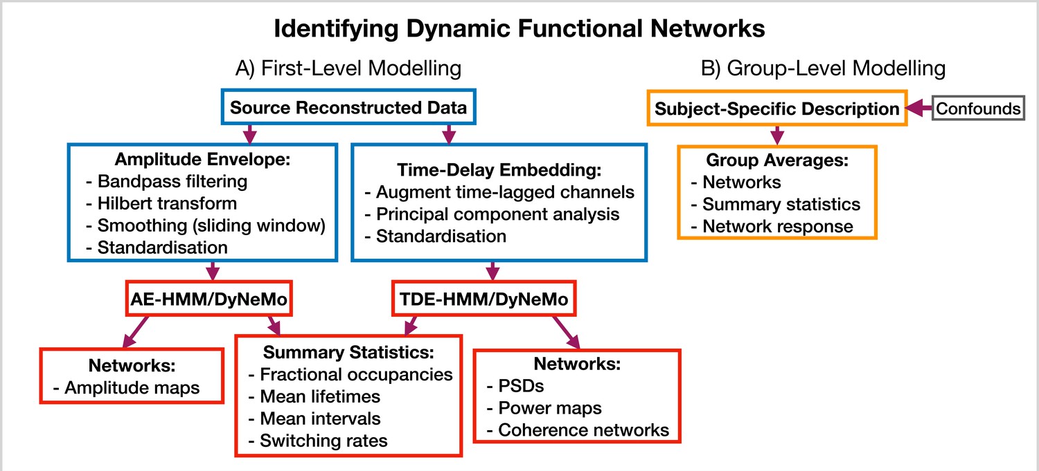
Dynamic functional network analysis pipeline.
(A) First-level modeling. This includes data preparation (shown in the blue boxes), model training, and post-hoc analysis (shown in the red boxes). The first-level modelling is used to derive subject-specific quantities. (B) Group-level modelling. This involves using the subject-specific description from the first-level modeling to model a group.
Figure 12
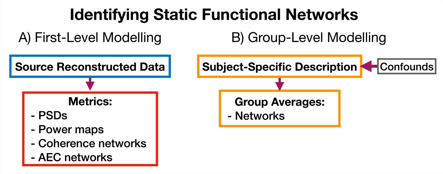
Static functional network analysis pipeline.
(A) The source reconstructed data is used to calculate metrics that describe networks. (B) The subject-specific metrics are used to model a group. Acronyms: Amplitude envelope correlation (AEC), Power spectral density (PSD).
Additional files
Download links
A two-part list of links to download the article, or parts of the article, in various formats.
Downloads (link to download the article as PDF)
Open citations (links to open the citations from this article in various online reference manager services)
Cite this article (links to download the citations from this article in formats compatible with various reference manager tools)
osl-dynamics, a toolbox for modeling fast dynamic brain activity
eLife 12:RP91949.
https://doi.org/10.7554/eLife.91949.3


