Movies reveal the fine-grained organization of infant visual cortex
- Department of Psychology, Stanford University, United States
- Department of Psychology, Columbia University, United States
- Department of Psychology, University of Pennsylvania, United States
- Department of Psychology, Yale University, United States
- Wu Tsai Institute, Yale University, United States
Figures
Figure 1 with 3 supplements
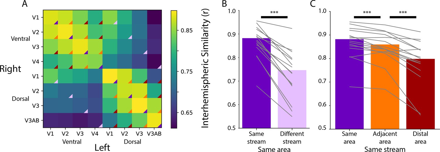
Homotopic correlations between retinotopic areas.
(A) Average correlation of the time course of activity evoked during movie-watching for all areas. This is done for the left and right hemisphere separately, creating a matrix that is not diagonally symmetric. The color triangles overlaid on the corners of the matrix cells indicate which cells contributed to the summary data of different comparisons in subpanels B and C. (B) Across-hemisphere similarity of the same visual area from the same stream (e.g. left ventral V1 and right ventral V1) and from different streams (e.g. left ventral V1 and right dorsal V1). (C) Across-hemisphere similarity in the same stream when matching the same area (e.g. left ventral V1 and right ventral V1), matching to an adjacent area (e.g. left ventral V1 and right ventral V2), or matching to a distal area (e.g. left ventral V1 and right ventral V4). Gray lines represent individual participants. ***=p<0.001 from bootstrap resampling.
Figure 1—figure supplement 1
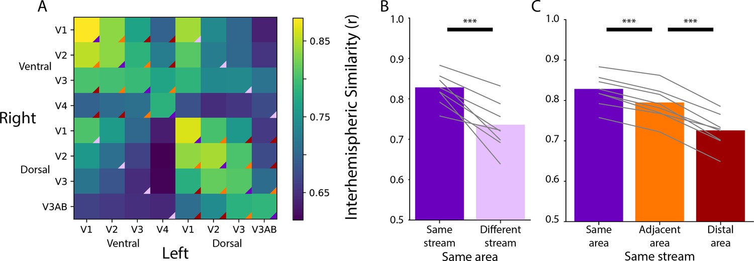
Homotopic correlations between retinotopic areas in the adult sample, akin to Figure 1.
(A) Average correlation of the time course of activity evoked during movie-watching for all areas. Correlation of homotopic areas: M=0.83 (range: 0.78–0.88). (B) Across-hemisphere similarity of the same visual area from the same stream and from different streams. Difference with bootstrap resampling: ΔFisher Z M=0.24, p<0.001. (C) Across-hemisphere similarity in the same stream when matching the same area, matching to an adjacent area, or matching to a distal area. Difference with bootstrap resampling: Same>Adjacent ΔFisher Z M=0.10, p<0.001; Adjacent>Distal ΔFisher Z M=0.16, p<0.001. Gray lines represent individual participants. ***=p<0.001 from bootstrap resampling.
Figure 1—figure supplement 2
Homotopic correlations when controlling for motion.
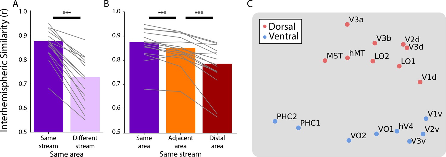
In this analysis, we computed correlations for all pairwise comparisons while partialing out our metric of motion: framewise displacement. In other words, if the functional time course in an area was correlated with the motion metric then this would decrease the correlation between that area and others. Subfigures A and B use task-evoked retinotopic definitions of areas (akin to Figure 1), whereas subfigure C uses anatomical definitions of areas (akin to Figure 2). Overall the results are qualitatively similar, suggesting that motion does not explain the effect observed here. (A) Correlation of the same area and same stream (e.g. left ventral V1 and right ventral V1) versus the same area and different stream (e.g. left ventral V1 and right dorsal V1). Difference with bootstrap resampling: ΔFisher Z M=0.43, p<0.001. (B) Correlation within the same stream between the same areas, adjacent areas (e.g. left ventral V1 and right ventral V2), or distal areas (e.g. left ventral V1 and right ventral hV4). Difference with bootstrap resampling: Same>Adjacent ΔFisher Z M=0.09, p<0.001; Adjacent>Distal ΔFisher Z M=0.20, p<0.001. Gray lines represent individual participants. ***=p<0.001 from bootstrap resampling. (C) Multi-dimensional scaling of the partial correlation between all anatomically defined areas. The time course of functional activity for each area was extracted and correlated across hemispheres, while partialing out framewise displacement. This matrix was averaged across participants and used to create a Euclidean dissimilarity matrix. MDS captured the structure of this matrix in two dimensions with suitably low stress (0.089). The plot shows a projection that emphasizes the similarity to the brain’s organization.
Figure 1—figure supplement 3
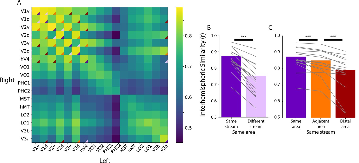
Homotopic correlations between anatomically defined areas corresponding to the data used in Figure 2.
(A) Average correlation of the time course of activity evoked during movie-watching for ventral and dorsal areas in an anatomical segmentation (Dale et al., 1999). This is done for the left and right hemispheres separately, which is why the matrix is not diagonally symmetric. The triangles overlaid on the matrix corner highlight the area-wise comparisons used in B and C. Only areas that we were able to retinotopically map (i.e. those that overlap with Figure 1) were used for this analysis. (B) Correlation of the same area and same stream (e.g. left ventral V1 and right ventral V1) versus the same area and different stream (e.g. left ventral V1 and right dorsal V1). Difference with bootstrap resampling: ΔFisher Z M=0.37, p<0.001. (C) Correlation within the same stream between the same areas, adjacent areas (e.g. left ventral V1 and right ventral V2), or distal areas (e.g. left ventral V1 and right ventral hV4). Difference with bootstrap resampling: Same>Adjacent ΔFisher Z M=0.09, p<0.001; Adjacent>Distal ΔFisher Z M=0.18, p<0.001. Gray lines represent individual participants. ***=p<0.001 from bootstrap resampling.
Figure 2 with 1 supplement
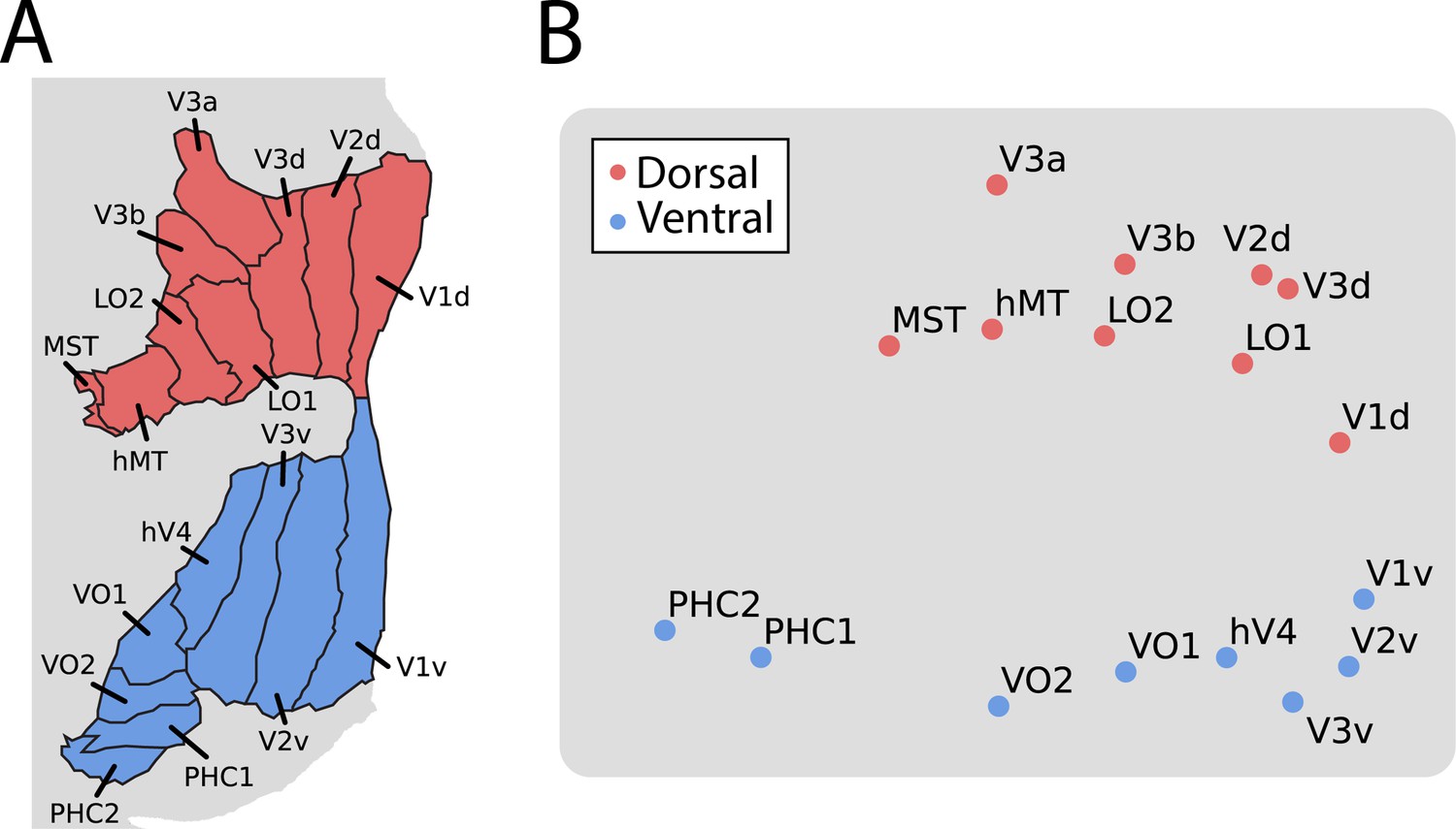
Multi-dimensional scaling (MDS) of movie-evoked activity in visual cortex.
(A) Anatomically defined areas Dale et al., 1999 used for this analysis, separated into dorsal (red) and ventral (blue) visual cortex, overlaid on a flatmap of visual cortex. (B) The time course of functional activity for each area was extracted and compared across hemispheres (e.g. left V1 was correlated with right V1). This matrix was averaged across participants and used to create a Euclidean dissimilarity matrix. MDS captured the structure of this matrix in two dimensions with suitably low stress. The plot shows a projection that emphasizes the similarity to the brain’s organization.
Figure 2—figure supplement 1
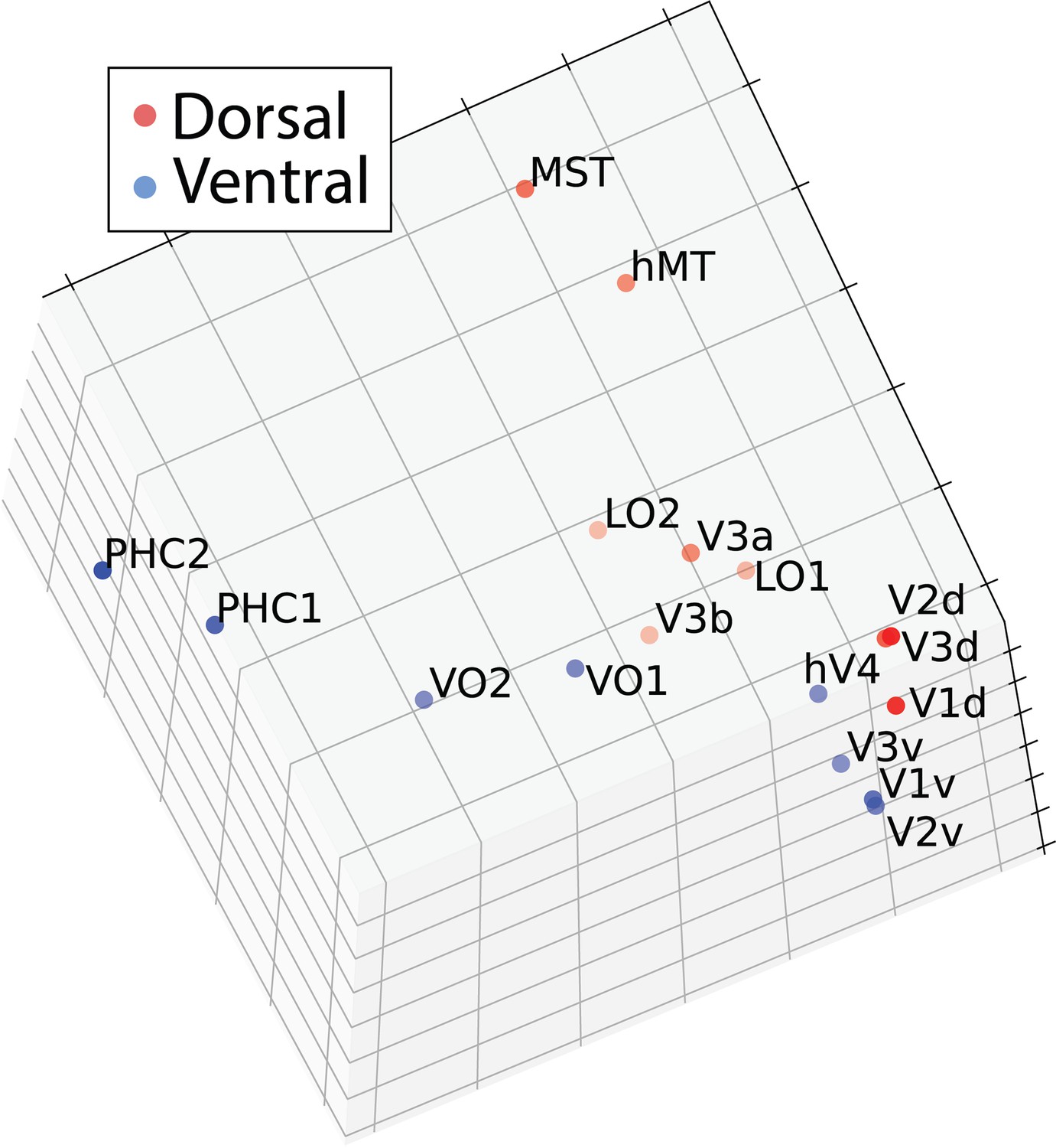
Multi-dimensional scaling of movie-evoked activity in adult visual cortex, akin to Figure 2.
A two-dimensional embedding had inappropriately high stress – 0.87 – whereas a three-dimensional embedding had appropriate stress: 0.105. This three-dimensional scatter depicts the similarity of the functional time course of areas as a function of Euclidean distance. The plot shows a projection that emphasizes the similarity to the brain’s organization.
Figure 3
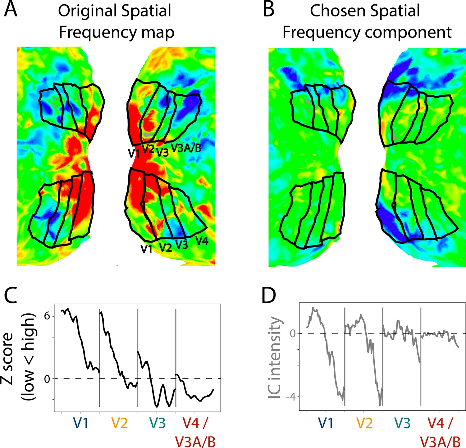
Example retinotopic task versus independent component analysis (ICA)-based spatial frequency maps.
(A) Spatial frequency map of a 17.1-month-old toddler. The retinotopic task data are from a prior study (Ellis et al., 2021). The view is of the flattened occipital cortex with visual areas traced in black. (B) Component captured by ICA of movie data from the same participant. This component was chosen as a spatial frequency map in this participant. The sign of ICA is arbitrary so it was flipped here for visualization. (C) Gradients in spatial frequency within-area from the task-evoked map in subpanel A. Lines parallel to the area boundaries (emanating from fovea to periphery) were manually traced and used to capture the changes in response to high versus low spatial frequency stimulation. (D) Gradients in the component map. We used the same lines that were manually traced on the task-evoked map to assess the change in the component’s response. We found a monotonic trend within area from medial to lateral, just like we see in the ground truth. This is one example result, find all participants in Figure 4—figure supplement 2.
Figure 4 with 3 supplements
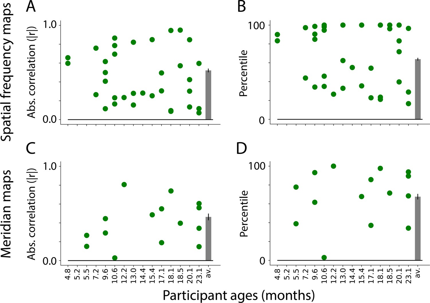
Similarity between visual maps from the retinotopy task and independent component analysis (ICA) applied to movies.
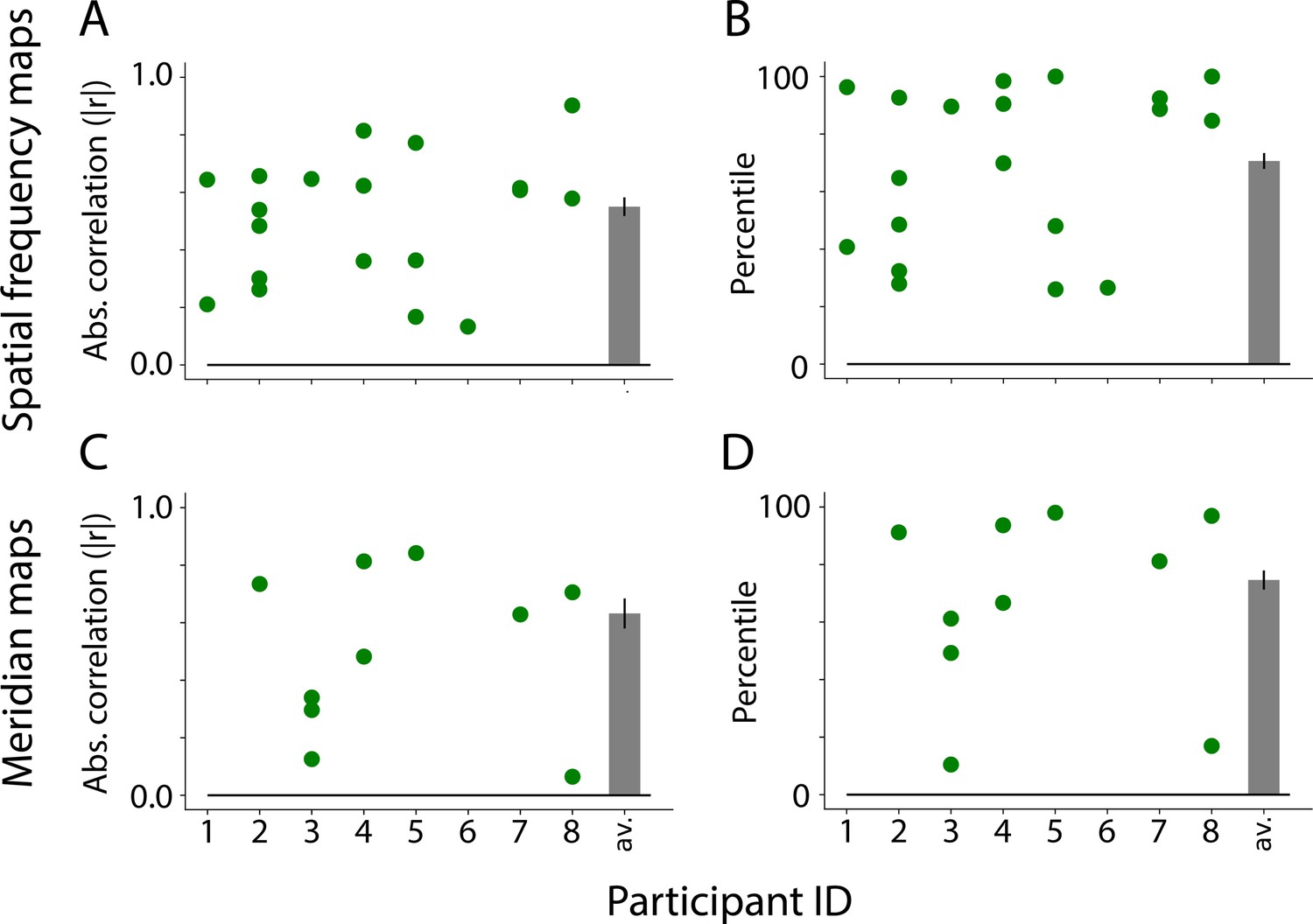
(A) Absolute correlation between the task-evoked and component spatial frequency maps (absolute values used because sign of ICA maps is arbitrary). Each dot is a manually identified component. At least one component was identified in 13 out of 15 participants. The bar plot is the average across participants. The error bar is the standard error across participants. (B) Ranked correlations for the manually identified spatial frequency components relative to all components identified by ICA. Bar plot is same as A. (C) Same as A but for meridian maps. At least one component was identified in 9 out of 15 participants. (D) Same as B but for meridian maps.
Figure 4—figure supplement 1
Similarity between visual maps from the adult retinotopy task and independent component analysis (ICA) applied to movies, akin to Figure 4.
(A) Absolute correlation between the task-evoked and component spatial frequency maps (absolute values used because sign of ICA maps is arbitrary). Each dot is a manually identified component. At least one component was identified in 8 out of 8 adult participants. The bar plot is the average across participants. The error bar is the standard error across participants. (B) Ranked correlations for the manually identified spatial frequency components relative to all components identified by ICA. Bar plot is same as A. Percentile tests: M=70.6 percentile, range: 26.6–92.3, ΔM from chance = 20.6, CI=[4.2–34.9], p=0.014. (C) Same as A but for meridian maps. At least one component was identified in 6 out of 8 participants. (D) Same as B but for meridian maps. Percentile tests: M=74.6 percentile, range: 40.3–98.0, ΔM from chance = 24.6, CI=[8.2–39.6], p=0.004.
Figure 4—figure supplement 2
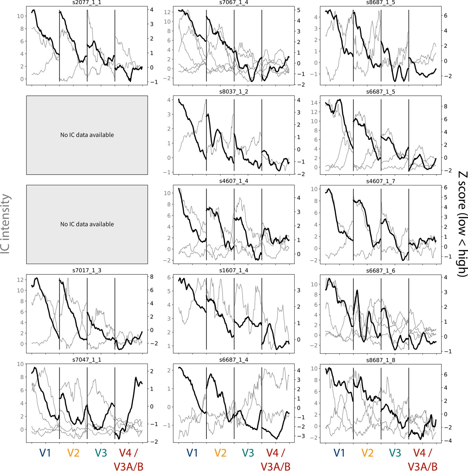
Gradients for the task-evoked and independent component analysis (ICA)-based spatial frequency maps.
The gray lines depict the gradients from each chosen IC map, and their scale is indicated by the Y-axis on the left-hand side. The sign of the maps has not been edited, but it is arbitrary. The black line indicates the gradient from the task-evoked map, and their scale is indicated by the Y-axis on the right-hand side. Participants are listed in order of age. Participant data is not reported if no components were chosen for that participant.
Figure 4—figure supplement 3
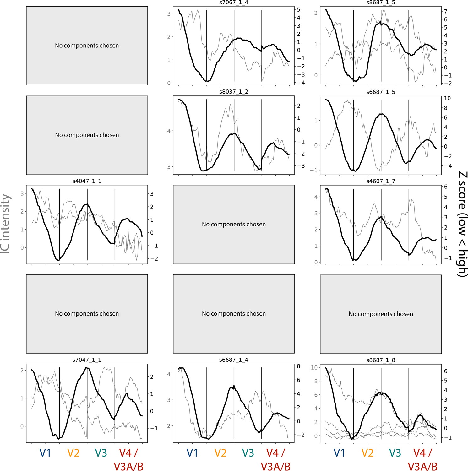
Gradients for the task-evoked and independent component analysis (ICA)-based meridian maps.
The gray lines depict the gradients from each chosen IC map, and their scale is indicated by the Y-axis on the left-hand side. The sign of the maps has not been edited, but it is arbitrary. The black line indicates the gradient from the task-evoked map, and their scale is indicated by the Y-axis on the right-hand side. Participants are listed in order of age. Participant data is not reported if no components were chosen for that participant.
Figure 5 with 1 supplement
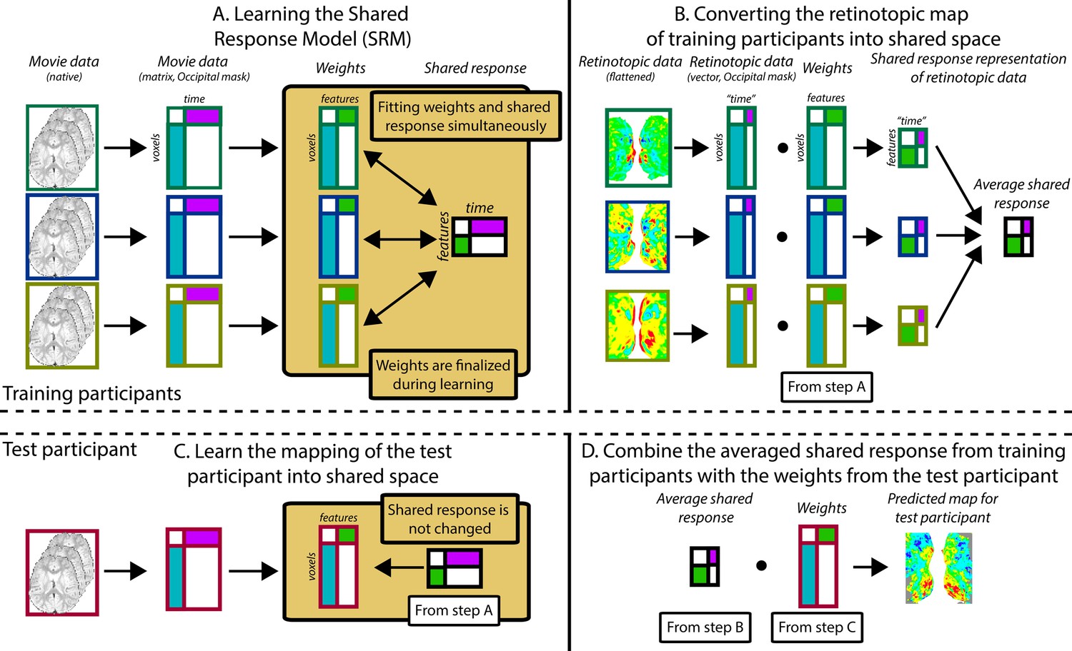
Pipeline for predicting visual maps from movie data.
The figure divides the pipeline into four steps. All participants watched the same movie. To predict infant data from other infants (or adults), one participant was held out of the training and used as the test participant. Step A: The training participants’ movie data (three color-coded participants shown in this schematic) is masked to include just occipital voxels. The resulting matrix is run through shared response modeling (SRM) (Chen et al., 2015) to find a lower-dimensional embedding (i.e. a weight matrix) of their shared response. Step B: The training participants’ retinotopic maps are transformed into the shared response space using the weight matrices determined in step A. Step C: Once steps A and B are finished, the test participant’s movie data are mapped into the shared space that was fixed from step A. This creates a weight matrix for this test participant. Step D: The averaged shared response of the retinotopic maps from step B is combined with the test participant’s weight matrix from step C to make a prediction of the retinotopic map in the test participant. This prediction can then be validated against their real map from the retinotopy task. Individual gradients for each participant are shown in Figure 6—figure supplement 2, Figure 6—figure supplements 3–5.
Figure 5—figure supplement 1

Cross-validation of the number of features in shared response modeling (SRM).
The movie data from all adult participants (Appendix 1—table 2) was split in half, with a 10 TR buffer between sets. The data were masked only to include occipital lobe voxels. The first half of the movie was used for training the SRM in all but one participant. The number of features learned by the SRM was varied across analyses from 1 to 25. The second half of the movie was then used to generate a shared response (i.e. the activity time course in each feature). To test the SRM, the held-out participant’s first half of data is used to learn a mapping of that participant into the SRM space (this mapping does not change the features learned and is not based on the second half of data). The second half of the held-out participant’s data is then mapped into the shared response space, like the other participants. Time-segment matching was performed on the shared response (Chen et al., 2015; Turek et al., 2018). In brief, time-segment matching tests whether a segment of the data (10 TRs) in the held-out participant can be matched to its correct timepoint based on the other participants. This tests whether the SRM succeeds in making the held-out participant similar to the others. This analysis was performed on each participant and movie separately (each has a line). The dashed line is chance for time-segment matching, averaged across all movies and participants. The black solid line at features = 10 reflects the number of features chosen.
Figure 6 with 5 supplements
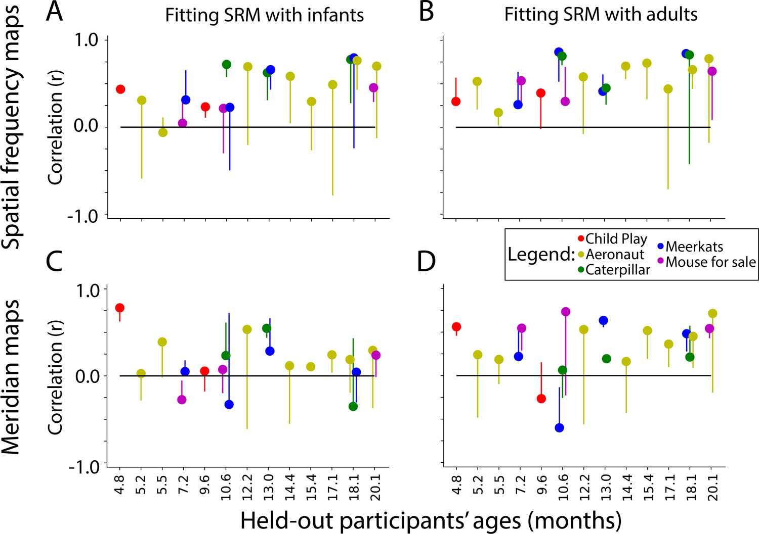
Similarity of shared response modeling (SRM)-predicted maps and task-evoked retinotopic maps.
Correlation between the gradients of the (A) spatial frequency maps and (C) meridian maps predicted with SRM from other infants and task-evoked retinotopy maps. (B, D) Same as A, except using adult participants to train the SRM and predict maps. Dot color indicates the movie used for fitting the SRM. The end of the line indicates the correlation of the task-evoked retinotopy map and the predicted map when using flipped training data for SRM. Hence, lines extending below the dot indicate that the true performance was higher than a baseline fit.
Figure 6—figure supplement 1
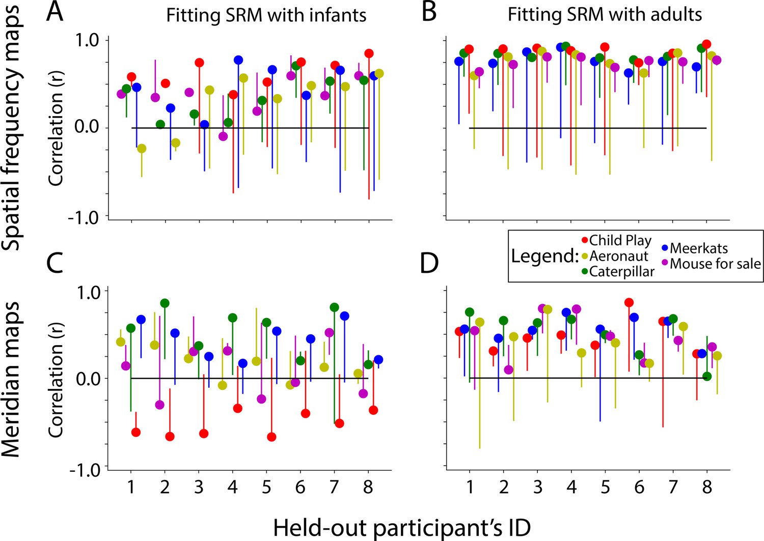
Similarity of shared response modeling (SRM)-predicted maps and task-evoked retinotopic maps in adults, akin to Figure 6.
Correlation between the gradients of the (A) spatial frequency maps and (C) meridian maps predicted with SRM from infants and their task-evoked retinotopy maps. Difference between real and flipped SRM fit: Spatial frequency=ΔFisher Z M=0.59, CI=[0.36–0.83], p<0.001. Meridian=ΔFisher Z M=−0.07, CI=[–0.22–0.10], p=0.382. Note: only two infants were used in the prediction with Child Play (red dots), hence why they likely show erratic behavior. (B, D) Same as A, except using adult participants to train the SRM and predict maps. Difference between real and flipped SRM fit: Spatial frequency=ΔFisher Z M=1.05, CI=[0.85–1.22], p<0.001. Meridian=ΔFisher Z M=0.49, CI=[0.36–0.64], p<0.001. Dot color indicates the movie used for fitting the SRM. The end of the line indicates the correlation of the task-evoked retinotopy map and the predicted map when using flipped training data for SRM.
Figure 6—figure supplement 2
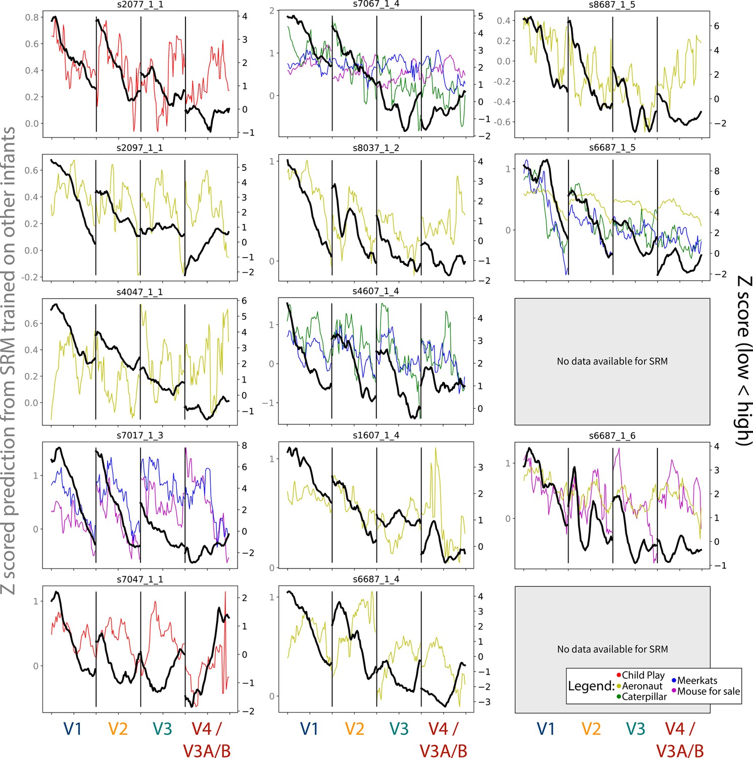
Gradients for the spatial frequency maps predicted using shared response modeling (SRM) from other infant participants, compared to the task-evoked gradients.
The colored lines depict the gradients from each chosen movie that could be used, and their scale is indicated by the Y-axis on the left-hand side. The black line indicates the gradient from the task-evoked map, and their scale is indicated by the Y-axis on the right-hand side. Participants are listed in order of age. Participant data is not reported if the participant did not have SRM-compatible movie data.
Figure 6—figure supplement 3
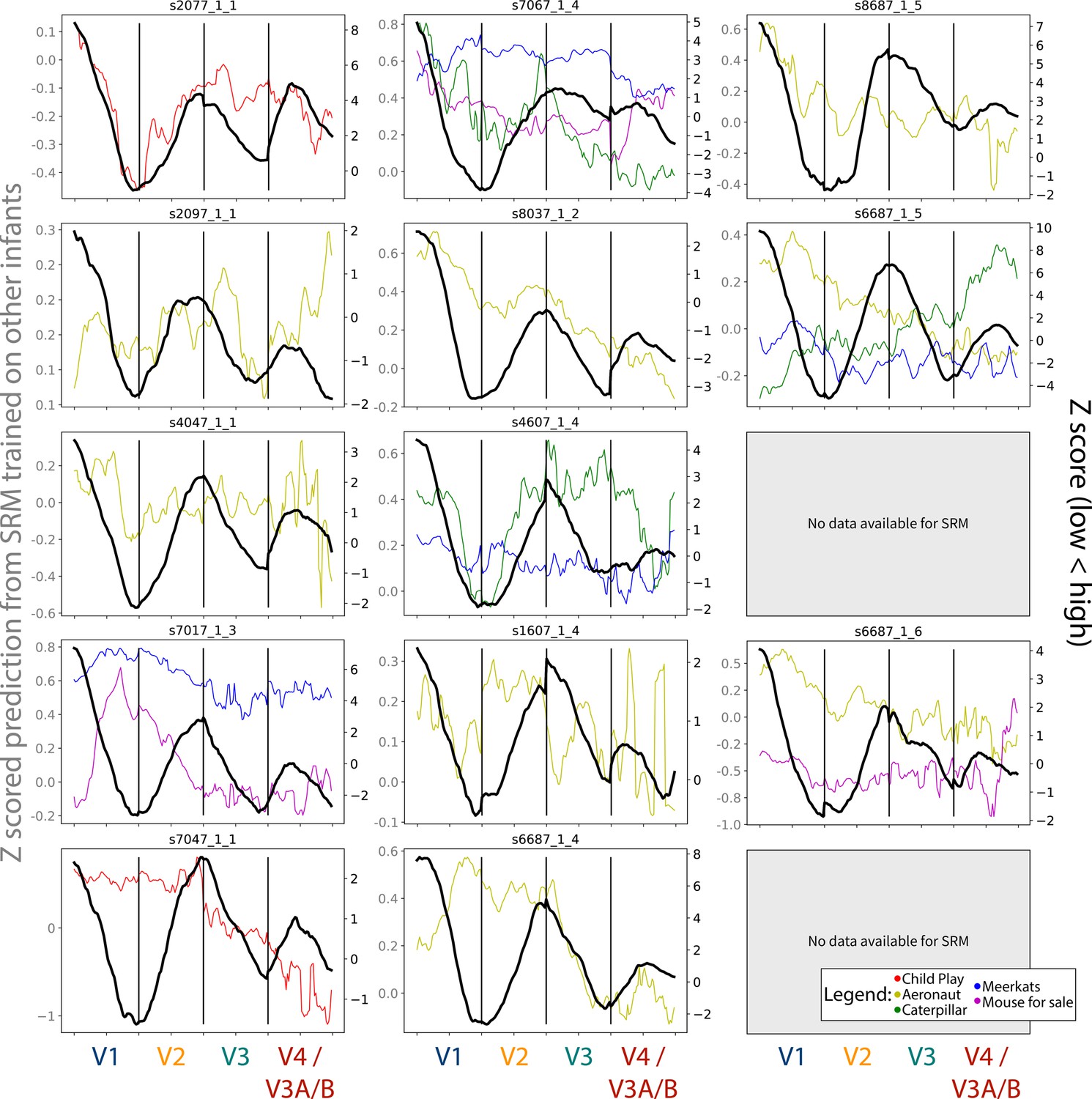
Gradients for the meridian maps predicted using shared response modeling (SRM) from other infant participants, compared to the task-evoked gradients.
The colored lines depict the gradients from each chosen movie that could be used, and their scale is indicated by the Y-axis on the left-hand side. The black line indicates the gradient from the task-evoked map, and their scale is indicated by the Y-axis on the right-hand side. Participants are listed in order of age. Participant data is not reported if the participant did not have SRM-compatible movie data.
Figure 6—figure supplement 4
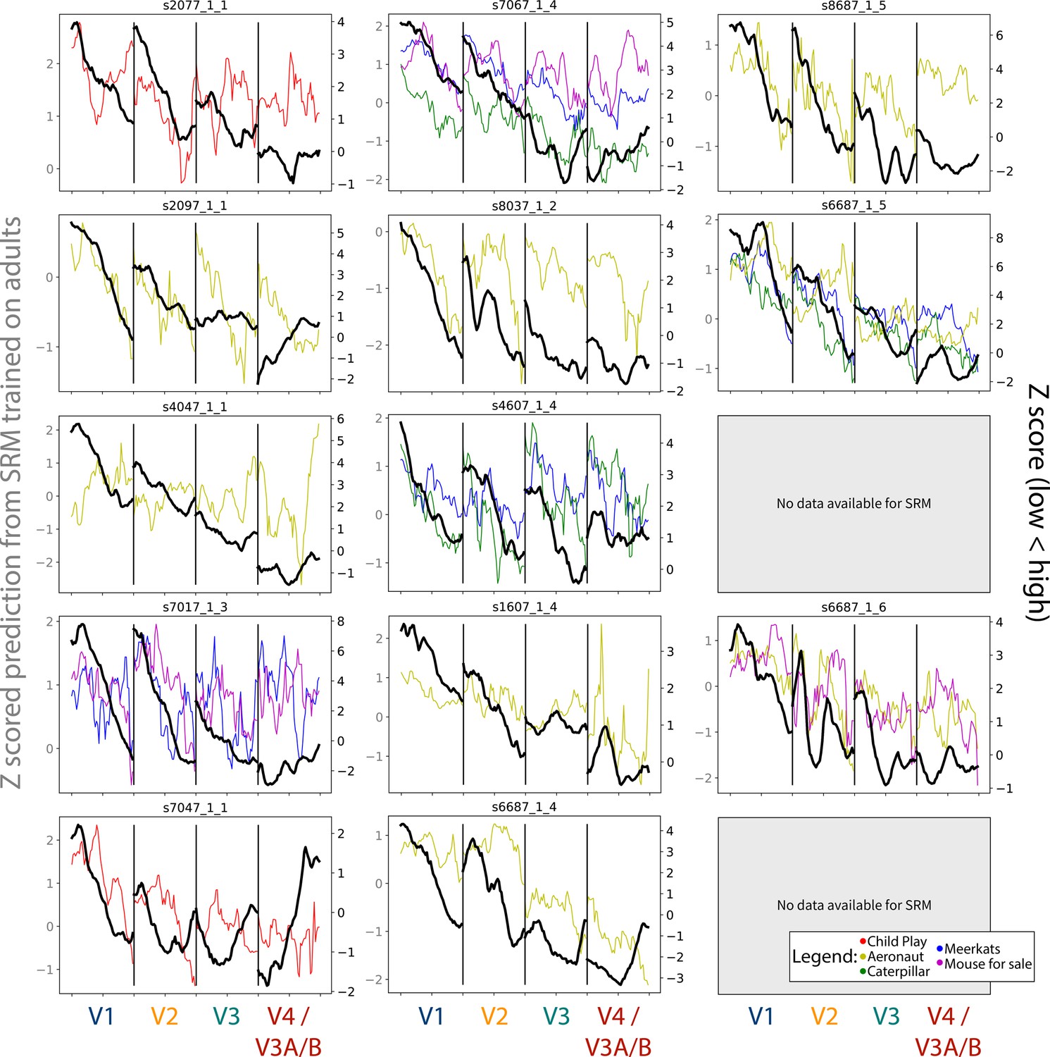
Gradients for the spatial frequency maps predicted using shared response modeling (SRM) from adult participants, compared to the task-evoked gradients.
The colored lines depict the gradients from each chosen movie that could be used, and their scale is indicated by the Y-axis on the left-hand side. The black line indicates the gradient from the task-evoked map, and their scale is indicated by the Y-axis on the right-hand side. Participants are listed in order of age. Participant data is not reported if the participant did not have SRM-compatible movie data.
Figure 6—figure supplement 5
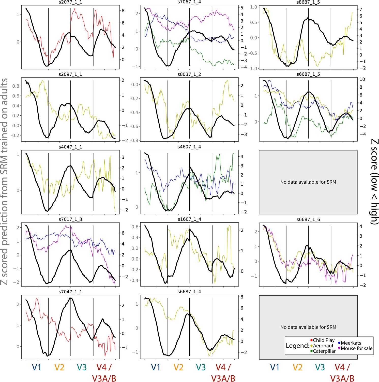
Gradients for the meridian maps predicted using shared response modeling (SRM) from adult participants, compared to the task-evoked gradients.
The colored lines depict the gradients from each chosen movie that could be used, and their scale is indicated by the Y-axis on the left-hand side. The black line indicates the gradient from the task-evoked map, and their scale is indicated by the Y-axis on the right-hand side. Participants are listed in order of age. Participant data is not reported if the participant did not have SRM-compatible movie data.
Tables
Key resources table
| Reagent type (species) or resource | Designation | Source or reference | Identifiers | Additional information |
|---|---|---|---|---|
| Software, algorithm | MATLAB v. 2017a | Mathworks, mathworks.com | RRID:SCR_001622 | |
| Software, algorithm | Psychtoolbox v. 3 | Medical Innovations Incubator, psychtoolbox.net/ | RRID:SCR_002881 | |
| Software, algorithm | Python v. 3.6 | Python Software Foundation, python.org | RRID:SCR_008394 | |
| Software, algorithm | FSL v. 5.0.9 | FMRIB, fsl.fmrib.ox.ac.uk/fsl/fslwiki | RRID:SCR_002823 | |
| Software, algorithm | Experiment menu v. 1.1 | Yale Turk-Browne Lab, (Ellis et al., 2020b) | https://github.com/ntblab/experiment_menu | |
| Software, algorithm | Infant neuropipe v. 1.3 | Yale Turk-Browne Lab, (Ellis et al., 2020c) | https://github.com/ntblab/infant_neuropipe |
Appendix 1—table 1
Demographic and dataset information for infant participants in the study.
‘Age’ is recorded in months. ‘Sex’ is the assigned sex at birth. ‘Retinotopy areas’ is the number of areas segmented from task-evoked retinotopy, averaged across hemispheres. Information about the movie data is separated based on analysis type: whereas all movie data is used for homotopy analyses and independent component analyses (ICA), a subset of data is used for shared response modeling (SRM). ‘Num.’ is the number of movies used. ‘Length’ is the duration in seconds of the run used for these analyses (includes both movie and rest periods). ‘Drops’ is the number of movies that include dropped periods. ‘Runs’ says how many runs or pseudoruns of movie data there were. ‘Gaze’ is the percentage of the data where the participants were looking at the movie.
| ID | Age | Sex | Retinotopy Areas | Homotopy and ICA | SRM | |||||
|---|---|---|---|---|---|---|---|---|---|---|
| Num. | Length | Drops | Runs | Gaze | Num. | Gaze | ||||
| s2077_1_1 | 4.8 | M | 6 | 1 | 430 | 0 | 1 | 97 | 1 | 97 |
| s2097_1_1 | 5.2 | M | 8 | 1 | 186 | 0 | 1 | 96 | 1 | 96 |
| s4047_1_1 | 5.5 | F | 7.5 | 1 | 186 | 0 | 1 | 99 | 1 | 99 |
| s7017_1_3 | 7.2 | F | 7 | 4 | 744 | 2 | 2 | 97 | 2 | 98 |
| s7047_1_1 | 9.6 | F | 7 | 1 | 432 | 0 | 1 | 91 | 1 | 91 |
| s7067_1_4 | 10.6 | F | 7.5 | 6 | 1110 | 3 | 2 | 98 | 3 | 99 |
| s8037_1_2 | 12.2 | F | 7.5 | 1 | 186 | 0 | 1 | 95 | 1 | 95 |
| s4607_1_4 | 13 | F | 7 | 3 | 558 | 1 | 1 | 93 | 2 | 90 |
| s1607_1_4 | 14.4 | M | 6 | 1 | 372 | 0 | 2 | 93 | 1 | 93 |
| s6687_1_4 | 15.4 | F | 8 | 1 | 186 | 0 | 1 | 82 | 1 | 82 |
| s8687_1_5 | 17.1 | F | 8 | 1 | 186 | 0 | 1 | 98 | 1 | 98 |
| s6687_1_5 | 18.1 | F | 8 | 5 | 930 | 2 | 2 | 94 | 3 | 92 |
| s4607_1_7 | 18.5 | F | 7.5 | 4 | 744 | 2 | 2 | 78 | 0 | NaN |
| s6687_1_6 | 20.1 | F | 6.5 | 6 | 1116 | 2 | 3 | 97 | 2 | 98 |
| s8687_1_8 | 23.1 | F | 7.5 | 4 | 744 | 2 | 1 | 97 | 0 | NaN |
| Mean | 13 | . | 7.3 | 2.7 | 540.7 | 0.9 | 1.5 | 93.7 | 1.3 | 94.5 |
Appendix 1—table 2
Number of participants per movie.
The first column is the movie name, where ‘Drop-’ indicates that it was a movie containing alternating epochs of blank screens. ‘SRM’ (shared response modeling) indicates whether the movie is used in SRM analyses. The movies that are not included in SRM are used for homotopy analyses and independent component analyses (ICA). ‘Ret. infants’ and ‘Ret. adults’ refers to the number of participants with retinotopy data that saw this movie. ‘Infant SRM’ and ‘Adult SRM’ refer to the number of additional participants available to use for training the SRM but who did not have retinotopy data. ‘Infant Ages’ is the average age in months of the infant participants included in the SRM, with the range of ages included in parentheses.
| Movie name | SRM | Ret. infants | Ret. adults | Infant SRM | Infant Ages | Adult SRM |
|---|---|---|---|---|---|---|
| Child_Play | 1 | 2 | 8 | 20 | 13.7 (3.3–32.0) | 9 |
| Aeronaut | 1 | 8 | 8 | 35 | 10.1 (3.6–20.1) | 32 |
| Caterpillar | 1 | 3 | 8 | 6 | 13.0 (6.6–18.2) | 0 |
| Meerkats | 1 | 4 | 8 | 6 | 13.4 (7.2–18.2) | 0 |
| Mouseforsale | 1 | 3 | 8 | 4 | 14.7 (7.2–20.1) | 0 |
| Elephant | 0 | 1 | 0 | 0 | 0 | |
| MadeinFrance | 0 | 1 | 0 | 0 | 0 | |
| Clocky | 0 | 1 | 0 | 0 | 0 | |
| Gopher | 0 | 1 | 0 | 0 | 0 | |
| Foxmouse | 0 | 2 | 0 | 0 | 0 | |
| Drop-Caterpillar | 0 | 4 | 0 | 0 | 0 | |
| Drop-Meerkats | 0 | 3 | 0 | 0 | 0 | |
| Drop-Mouseforsale | 0 | 1 | 0 | 0 | 0 | |
| Drop-Elephant | 0 | 1 | 0 | 0 | 0 | |
| Drop-MadeinFrance | 0 | 1 | 0 | 0 | 0 | |
| Drop-Clocky | 0 | 2 | 0 | 0 | 0 | |
| Drop-Ballet | 0 | 1 | 0 | 0 | 0 | |
| Drop-Foxmouse | 0 | 1 | 0 | 0 | 0 |
Appendix 1—table 3
Details for each movie used in this study.
‘Name’ specifies the movie name. ‘Duration’ specifies the duration of the movie in seconds. Movies were edited to standardize length and remove inappropriate content. ‘Sound’ is whether sound was played during the movie. These sounds include background music, animal noises, and sound effects, but no language. ‘Description’ gives a brief description of the movie, as well as a current link to it when appropriate. All movies are provided in the data release.
| Name | Duration | Sound | Description |
|---|---|---|---|
| Child_Play | 406 | 0 | Four photo-realistic clips from `Daniel Tiger' showing children playing. The clips showed the following: 1. children playing in an indoor playground (84 s); 2. a family making frozen banana desserts (64 s); 3. a child visiting the doctor (115 s); 4. children helping with indoor and outdoor chores (143 s). |
| Aeronaut | 180 | 0 | A computer-generated segment from a short film titled ”Soar'' (https://vimeo.com/148198462) and described here (Yates et al., 2022). |
| Caterpillar | 180 | 1 | A computer-generated segment from a short film titled ”Sweet Cocoon'' (https://www.youtube.com/watch?v=yQ1ZcNpbwOA). This video depicts a caterpillar trying to fit into its cocoon so it can become a butterfly. |
| Meerkats | 180 | 1 | A computer-generated segment from the short film titled ”Catch It'' (https://www.youtube.com/watch?v=c88QE6yGhfM). It depicts a gang of meerkats who take back a treasured fruit from a vulture. |
| Mouse for Sale | 180 | 1 | A computer-generated segment from a short film of the same name (https://www.youtube.com/watch?v=UB3nKCNUBB4). It shows a mouse in a pet store who is teased for having big ears. |
| Elephant | 180 | 1 | A computer-generated segment from a short film of the same name (https://www.youtube.com/watch?v=h_aC8pGY1aY). It shows an elephant in a china shop. |
| Made in France | 180 | 1 | A computer-generated segment from a short film of the same name (https://www.youtube.com/watch?v=Her3d1DH7yU). It shows a mouse making cheese. |
| Clocky | 180 | 1 | A computer-generated segment from a short film of the same name (https://www.youtube.com/watch?v=8VRD5KOFK94). It shows a clock preparing to wake up its owner. |
| Gopher | 180 | 1 | A computer-generated segment named `Gopher broke' (https://www.youtube.com/watch?v=tWufIUbXubY). It shows a gopher collecting food. |
| Foxmouse | 180 | 1 | A computer-generated segment named `The short story of a fox and a mouse' (https://www.youtube.com/watch?v=k6kCwj0Sk4s). It shows a fox playing with a mouse in the snow. |
| Ballet | 180 | 1 | A computer-generated segment named `The Duet' (https://www.youtube.com/watch?v=GuX52wkCIJA). This is an artistic rendition of growing up and falling in love. |
Appendix 1—table 4
Correlations between infant gradients and the spatial average of other infants or adults.
For each participant, all other participants with retinotopy data (adults or infants) were aligned to standard surface space and averaged. The traced lines from the held-out participant were then applied to this average. The resulting gradients were correlated with the held-out participant and the correlation is reported here. This was done separately for meridian maps and spatial frequency maps.
| ID | Adults | Infants | ||
|---|---|---|---|---|
| Spatial freq. | Meridians | Spatial freq. | Meridians | |
| s2077_1_1 | 0.85 | 0.77 | 0.89 | 0.81 |
| s2097_1_1 | 0.66 | 0.72 | 0.66 | 0.65 |
| s4047_1_1 | 0.86 | 0.78 | 0.94 | 0.82 |
| s7017_1_3 | 0.9 | 0.92 | 0.93 | 0.92 |
| s7047_1_1 | 0.43 | 0.65 | 0.56 | 0.64 |
| s7067_1_4 | 0.87 | 0.67 | 0.92 | 0.61 |
| s8037_1_2 | 0.92 | 0.73 | 0.93 | 0.83 |
| s4607_1_4 | 0.77 | 0.97 | 0.74 | 0.94 |
| s1607_1_4 | 0.93 | 0.82 | 0.92 | 0.86 |
| s6687_1_4 | 0.87 | 0.9 | 0.93 | 0.93 |
| s8687_1_5 | 0.97 | 0.89 | 0.98 | 0.83 |
| s6687_1_5 | 0.92 | 0.81 | 0.97 | 0.91 |
| s4607_1_7 | 0.85 | 0.91 | 0.8 | 0.86 |
| s6687_1_6 | 0.92 | 0.94 | 0.86 | 0.97 |
| s8687_1_8 | 0.89 | 0.93 | 0.9 | 0.88 |
| Mean | 0.84 | 0.83 | 0.86 | 0.83 |
Additional files
Download links
A two-part list of links to download the article, or parts of the article, in various formats.
Downloads (link to download the article as PDF)
Open citations (links to open the citations from this article in various online reference manager services)
Cite this article (links to download the citations from this article in formats compatible with various reference manager tools)
Movies reveal the fine-grained organization of infant visual cortex
eLife 12:RP92119.
https://doi.org/10.7554/eLife.92119.4


