Sequentially activated discrete modules appear as traveling waves in neuronal measurements with limited spatiotemporal sampling
- School of Neurobiology, Biochemistry, and Biophysics, Tel Aviv University, Israel
- School of Physics & Astronomy, Faculty of Exact Sciences, Tel Aviv University, Israel
- Sagol School of Neuroscience, Tel Aviv University, Israel, Israel
Figures
Figure 1 with 1 supplement
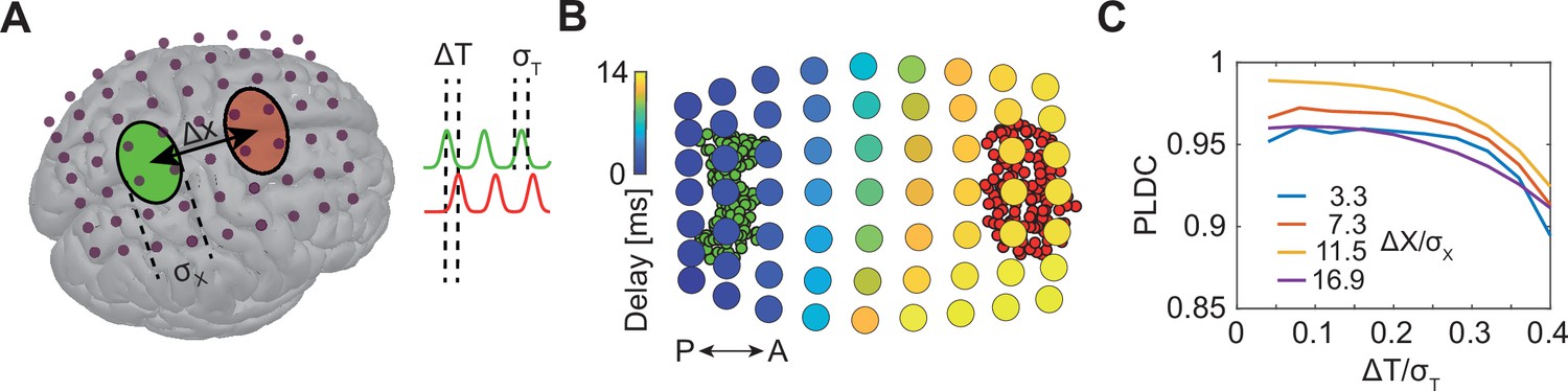
Sequential activation of two discrete brain areas appears as waves in simulated EEG phase latency maps.
(A) Schematic illustration of simulated EEG. Two brain areas (green and red ellipses) are defined on the cortex by a set of dipoles that are activated uniformly with a time delay (ΔT) between areas. A finite element forward model in Brainstorm (Tadel et al., 2011) is used to simulate the resulting potentials measured with EEG electrodes (purple dots). (B) Latency to peak measured across electrodes following the sequential activation of two sets of dipoles (green and red circles in the background) with a distance of 11 cm (Δx/σx=16.9) and time delay of 20 ms (ΔT/σT=0.2). A continuous delay pattern propagating from posterior (P) to anterior (A) is observed. (C) Phase latency distance correlations (PLDCs) for different distances and different delays between two activated areas. PLDC remains close to 1 (indicating apparent wave propagation) for a wide range of values.
Figure 1—figure supplement 1
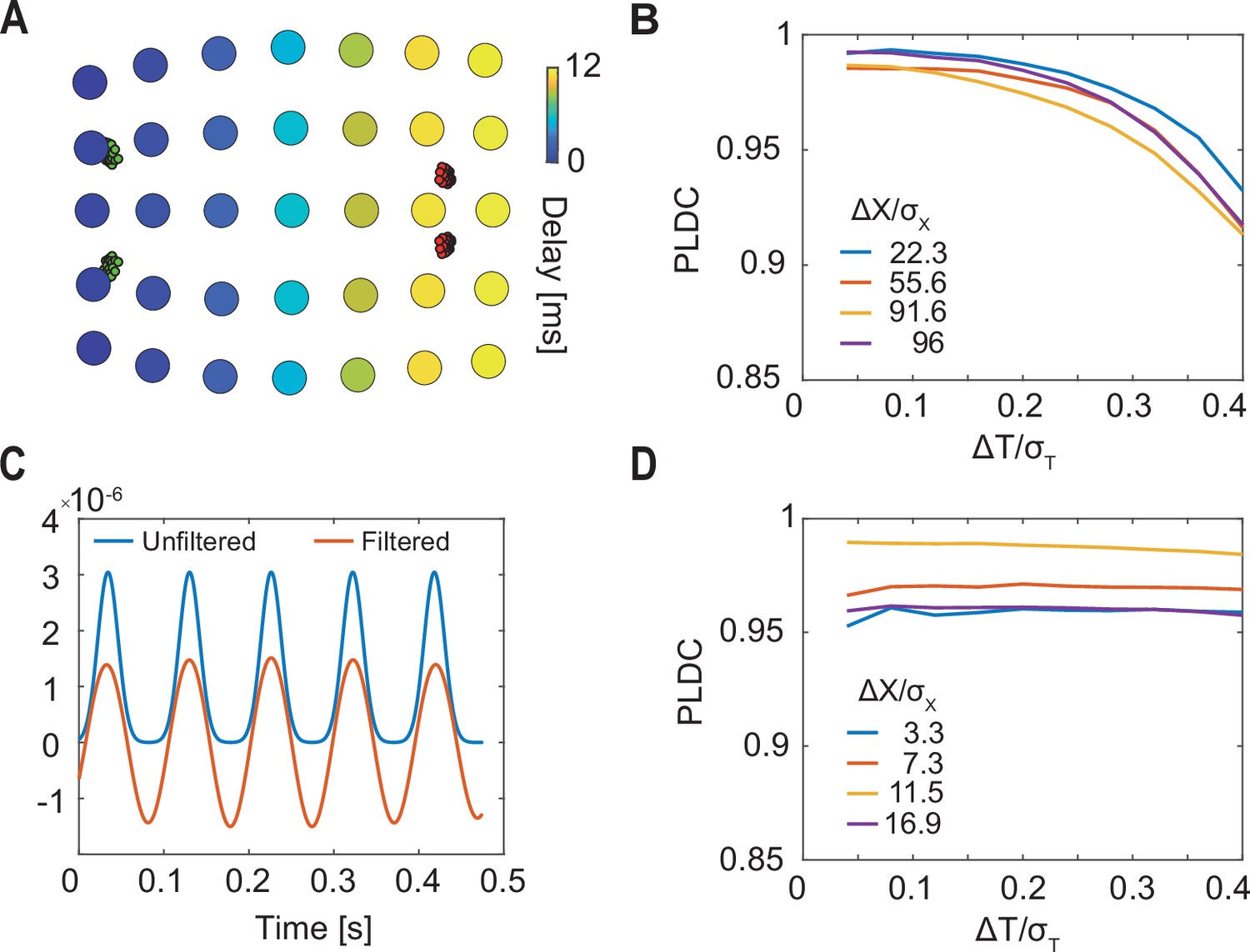
Sequential activation of two discrete small brain areas appears as waves in simulated EEG phase latency maps.
(A) Latency to peak as measured across electrodes following the sequential activation of two sets of localized dipoles (green and red, as in Figure 1B) simulating the activation of small cortical areas. A wave-like delay pattern is observed. (B) Phase latency distance correlations (PLDCs) for different distances and different delays between two activated areas (as in Figure 1C). PLDC remains close to 1 (indicating wave propagation) for a wide range of values. (C) Activation dynamics before and after filtering into a narrow-band frequency range (10–12 Hz). (D) PLDC for two sequentially activated large areas (as in Figure 1C) after narrow-band filtering (C). Filtering increases PLDC values making rendering them more wave-like.
Figure 2 with 5 supplements
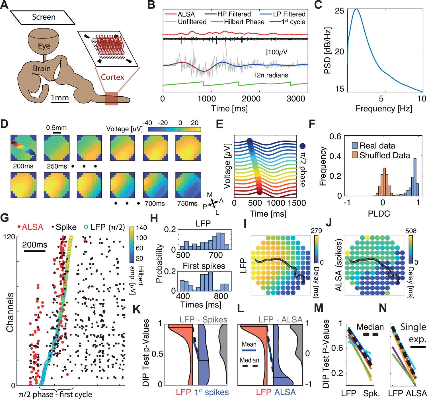
Sequential activation of discrete spiking populations underlies local field potential (LFP) waves in turtle cortex.
(A) Schematic of the experimental setup. The brain with eye attached is extracted and the visual cortex is flattened on a multi-electrode array (MEA) and its activity is measured in response to visual stimulation of the retina. (B) A cortical response following visual stimulation at t=0. Traces show the following data: raw electrode (gray), low-pass filtered (<2 Hz, blue with dotted line marking the first oscillation cycle), high-pass filtered (>200 Hz, black), average local spiking activity (ALSA) (red), and the instantaneous phase of the low-pass filtered trace (green). (C) Power spectral density (averaged over 1000 randomly selected trials from one experiment). (D) Dynamics of low-pass filtered (<2 Hz) and averaged (n=4000) cortical responses to visual stimulation. The amplitude in each time window (200–750 ms post-stimulus in 50 ms intervals) is color-coded and presented on the physical space of the electrode. Filled color-coded circles mark the electrodes recorded in (E). M=medial, A=anterior, L=lateral, P=posterior. (E) Averaged (n=4000) low-pass filtered (<2 Hz) traces for channels along the delay gradient. The maximum is marked by a circle and its location on the array is color-coded in (D). (F) Phase latency distance correlation (PLDC) distribution for all trials with strong waves (n=2415, blue) from this experiment and for the same trials with shuffled latencies (red). (G) Spiking responses (black dots) in a single visual stimulation trial. Empty circles mark the π/2 phase crossing. Red circles denote the ALSA onset for each electrode. Electrodes were reordered according to the LFP phase crossings. (H) The distribution of LFP phase crossing times and first spike times for the response in (G) with corresponding DIP values (0.85 and 0.0002, respectively). (I–J) Latency maps on the electrode array’s physical space extracted from the Hilbert phase (I) and ALSA (J). Black line denotes the wave center path extracted from the Hilbert phase (see Methods). (K) DIP test p-value distribution of the first spikes (blue), Hilbert phase crossings (red), and differences between both per trial (gray) for strong waves with enough spikes (n=902). Distribution medians (solid black line) are connected by a dashed black line (blue line connects the distributions’ means). (L) Same as (K) but for ALSA. (M, N) Medians of the DIP test p-values (black lines in K, L, respectively) from six recordings in four animals. Dashed black line marks the median over all experiments. All results except (N, M) are from the same recording.
Figure 2—figure supplement 1
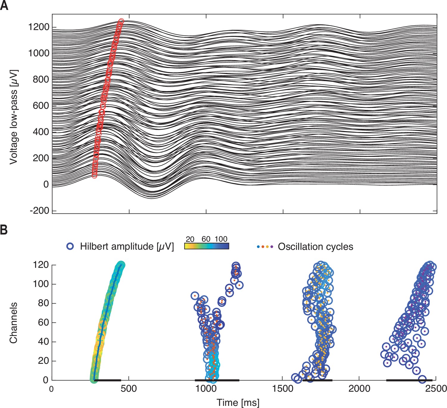
Identification of waves during single oscillation cycles.
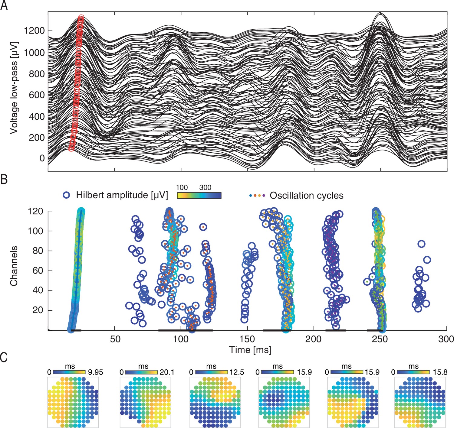
(A) The low-pass filtered (0–2 Hz) voltage responses across all electrodes to a single visual stimulation. Red circle marks the same oscillation phase across electrodes. Traces of different electrodes are displaced along the y axis. (B) Single cycles are identified (colored center dots with different colors marking different cycles) from the filtered traces in (A). Within each cycle, the oscillation phase is marked by empty circles with color-coded amplitude. Channels in (A, B) are reordered according to the phase time of the first oscillation cycle. Cycle durations are marked by black lines at the bottom.
Figure 2—figure supplement 2
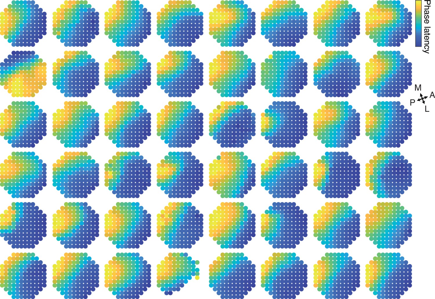
Phase latency maps of single trials.
The phase latency is plotted on the physical space of the electrodes for the first oscillation cycle in 48 single trials. Color code is normalized between maximum and minimum for every trial. The strongest events with most electrode participating in the first oscillation cycle were used. Electrodes that did not participate in a specific oscillation event (see oscillation cycle detection method) were not plotted.
Figure 2—figure supplement 3

Spikes are locked to the 0–2 Hz oscillation.
(A) The distribution for the first spikes to the visual stimulation relative to the 0–2 Hz oscillation. (B, C) Same as (A) but for average local spiking activity (ALSA) onset times (B) and for all spikes during all cycles in the recording (C). Notice that both the spikes and ALSA exhibit a similar locking with the ALSA distribution being narrower. Shown above is the mode of the distribution calculated over 36 bins with width of π/18.
Figure 2—figure supplement 4
DIP statistics captures segregation of propagating activity into modules.
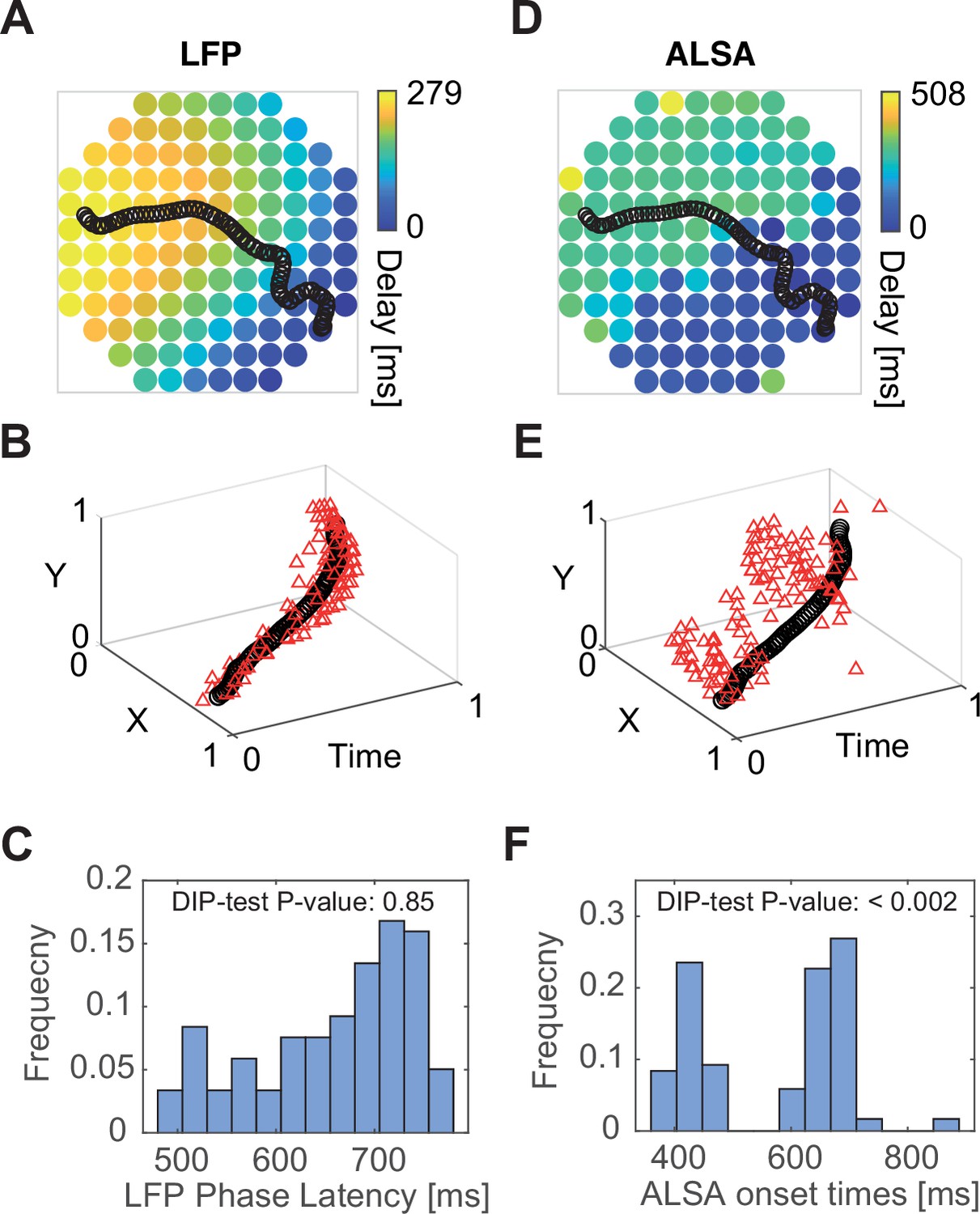
(A) Phase latency map for the local field potential (LFP) in the trial shown in Figure 2G. The wave center path is shown in black. (B) Single trial’s phase crossing events (red triangle) plotted together with the wave center path (black) as points in three-dimensional space (two spatial coordinates representing the electrode layout and one temporal coordinate). (C) The distribution of phase delays in time and the corresponding DIP test value for this distribution. (D–F) Same as (A–C) but for average local spiking activity (ALSA) onset times. While the LFP phase crossings (A–C) are spread around the wave center path in space and time, the ALSA onset times are organized as clustered groups. Correspondingly, the DIP value for the LFP is considerably higher than for ALSA. Panels A, C, D, F are identical to panels H, I, J in Figure 2, but shown here for comparison.
Figure 2—figure supplement 5
Identification of waves for single oscillation cycles in the β-band.
(A) The bandpass filtered (12–35 Hz) voltage responses across all electrodes to a single visual stimulation. Red circle marks the same oscillation phase across electrodes. Traces of different electrodes are displaced along the y axis. (B) Single cycles are identified (colored center dots with different colors marking different cycles) from the filtered traces in (A). (B) Single cycles are identified (color dots with different colors marking different cycles; cycle durations are marked by black lines) from the filtered traces in (A). Within each cycle, the oscillation phase is marked by empty circles with color-coded amplitude. Channels in (A, B) are reordered according to the phase time of the first oscillation cycle. Cycle durations are marked by black lines at the bottom (events with less than 100 of 120 active channels were excluded from analysis). (C) Examples of phase latency maps extracted from single waves in the 12–35 Hz band.
Figure 3 with 1 supplement
A simple analytic model of sequentially activated Gaussians exhibits traveling peaks with a diversity of patterns.
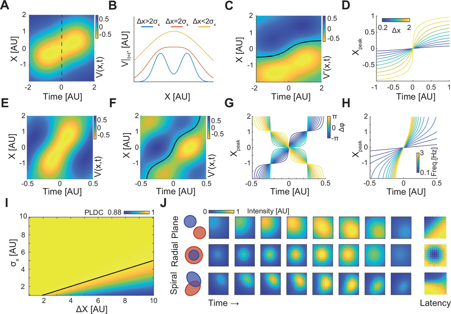
(A) The spatiotemporal potential of two sequentially activated one-dimensional spatial Gaussians (centers; x1=−0.5 and x2=0.5; standard deviation σx=1), each with a temporal Gaussian activation profile (peaking at t1=–1 and t2=1; standard deviation σt=1), as in Equation 1. Notice wave-like propagation. (B) Spatial profile of Equation 1 at time t = (t1+t2)/2 (dotted line in (A)) for three conditions. Notice that for Δx≤2σx the spatial profile is concave. (C) The spatial derivative of V(x,t) in (A). Black line marks Gaussian peak dynamics (zero crossing points of the spatial derivative). (D) Peak dynamics for different values of distances between Gaussian centers (Δx). Notice that the average velocity increases with Δx. (E, F) Same as in (A, C) but for a model of a periodically fluctuating Gaussian (Equation 3) (x1=−0.5, x2=0.5, σx=1, f=1, ϕ1=-3π/8, ϕ2=3π/8). (G, H) The peak dynamics (as in (D)) for the model in (E, F) as a function of the phase difference between Gaussians, Δϕ (G), and f, the frequency of the oscillation (H). f=1 in (G) and ϕ1=-π/4, ϕ2=π/4 in (H). Notice that wave velocity increases with frequency and can change sign as a function of Δϕ. (I) Phase latency-distance correlation (PLDC) values calculated for different Δx and σx. Black line marks the Δx=2σx border. (J) Plane, radial, and spiral-like propagation patterns and the resulting phase latency maps (right) for different spatial arrangements of two sequentially activated Gaussians (left).
Figure 3—video 1
Dynamics of two consecutively activated Gaussians.
The amplitude (AU) of two sequentially activated Gaussians is shown as a function of time (according to Equation 1). The distance between Gaussian centers was Δx=2σx (left) and Δx=3σx (right) (σx being the standard deviation) and Δt=σt. Superimposed is the calculated optical flow (calculated using the Horn-Schunck method) showing propagation along the path between the two Gaussians.
Additional files
Download links
A two-part list of links to download the article, or parts of the article, in various formats.
Downloads (link to download the article as PDF)
Open citations (links to open the citations from this article in various online reference manager services)
Cite this article (links to download the citations from this article in formats compatible with various reference manager tools)
Sequentially activated discrete modules appear as traveling waves in neuronal measurements with limited spatiotemporal sampling
eLife 12:RP92254.
https://doi.org/10.7554/eLife.92254.3


