Figures and data in A parameterized two-domain thermodynamic model explains diverse mutational effects on protein allostery

Figures
Tables
Additional files

5 figures, 2 tables and 1 additional file

Figures

Figure 1

Download asset Open asset

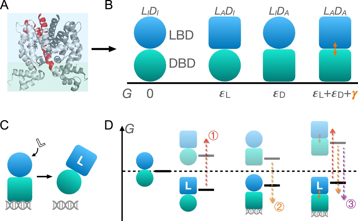
Schematic illustration of the two-domain statistical thermodynamic model of TetR allostery.

(A) The crystal structure of TetR(B) in complex with minocycline and magnesium (PDB code: 4AC0). The red residues are the hotspots identified in the deep mutational scanning (DMS) study (Leander et al., 2020). (B) Four possible conformations of a two-domain TetR molecule with their corresponding free energies ( $G$ ). $G$ of the $L_{I} D_{I}$ state is set to 0. Blue/green circle (square) denotes the inactive (active) state of ligand/DNA-binding domain (LBD/DBD). (C) A simple repression scheme of TetR function. Binding of the ligand (inducer) favors the inactive state of DBD in TetR, which then releases the DNA operator and enables the transcription of the downstream gene. (D) Schematic free energy diagram of the possible binding states of TetR at fixed ligand and operator concentrations. Red, orange, and purple arrows show how a mutation can disrupt allostery by (1) increasing $ε_{L}$ ; (2) decreasing $ε_{D}$ , and (3) decreasing $γ$ . The L- $L_{A} D_{A}$ state is not explicitly shown in the last column as the doubly bound L- $L_{A} D_{A}$ -D state is expected to have a lower free energy. Note that mutations that change the binding affinities of the active LBD/DBD to ligand/operator are not discussed here as we focus on the intrinsic allosteric properties of the transcription factor (TF) itself.

Figure 2 with 3 supplements

Download asset Open asset

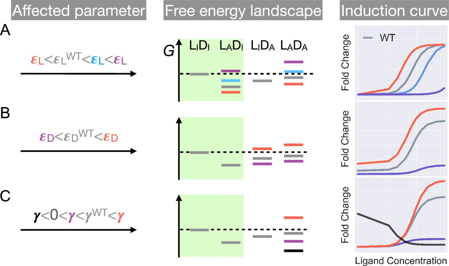
Schematic illustration of the characteristic effects of perturbations in the three biophysical parameters on the free energy landscape and the corresponding induction curves of a two-domain allosteric system.

Panels A, B, and C illustrate how changing $ε_{L}$ , $ε_{D}$ , and $γ$ alone affects the free energy landscape for the binding states shown in Figure 1D and the induction curve. For the black induction curve in (C), the values of $ε_{L}$ and $ε_{D}$ are also adjusted to aid visualization of the negative monotonicity of the gene expression level (fold change) as a function of ligand concentration. The green shade in the middle column separates the DNA-bound states from the rest. In the free energy landscapes shown in the middle column, ligand or DNA binding is always assumed when the corresponding domain is in the active conformation.

Figure 2—figure supplement 1

Download asset Open asset

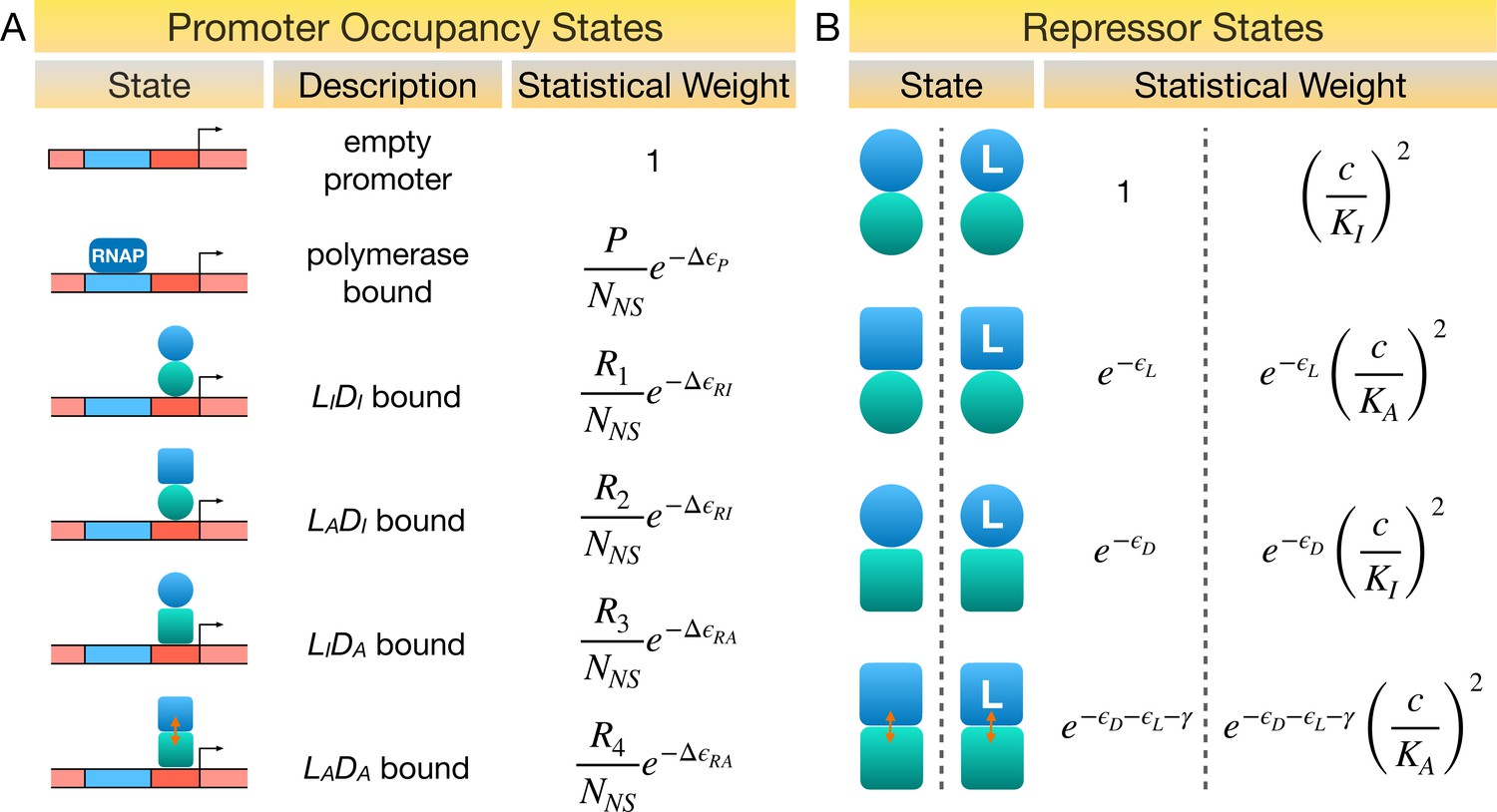
Statistical weights of promoter occupancy states and repressor states.

(A) Statistical weights of the promoter occupancy states, with the empty promoter state taken as reference. P is the average number of RNA polymerase (RNAP) per cell. $R_{1}, R_{2}, R_{3}, a n d R_{4}$ denote the average number of repressors in the $L_{I} D_{I}, L_{A} D_{I}, L_{I} D_{A}, a n d L_{A} D_{A}$ state per cell, respectively. N_NS is the number of non-specific DNA-binding sites in the cell. $Δ ε_{P}, Δ ε_{R A}, a n d Δ ε_{R I}$ represent the energy differences between specific and non-specific DNA binding of RNAP, repressor with DNA-binding domain (DBD) in the active and inactive conformations, respectively. (B) Statistical weights of the allosteric states of the repressor, with the $L_{I} D_{I}$ state taken as reference. $K_{A}$ and $K_{I}$ are the dissociation constants of ligand to the repressor with ligand-binding domain (LBD) in the active and inactive conformations, respectively, and c is ligand concentration. Partial binding of ligand is ignored in the symmetric model. All energy terms in the exponents are evaluated in the unit of $k_{B} T$ .

Figure 2—figure supplement 2

Download asset Open asset

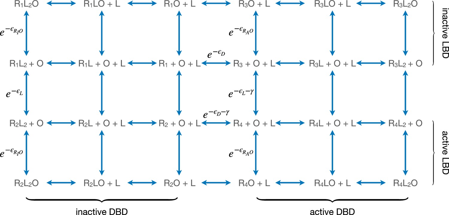
Equilibria among different conformational and binding states of the repressor.

Here, L and O represent ligand and operator respectively. $ε_{R_{A} O} a n d ε_{R_{I} O}$ are the free energies of operator binding for repressor with DNA-binding domain (DBD) in the active and inactive conformation, respectively. R₁, R₂, R₃, and R₄ denote the $L_{I} D_{I}, L_{A} D_{A}, L_{I} D_{A}, a n d L_{A} D_{A}$ state of the repressor, respectively. All energy terms in the exponents are evaluated in the unit of k_BT.

Figure 2—figure supplement 3

Download asset Open asset

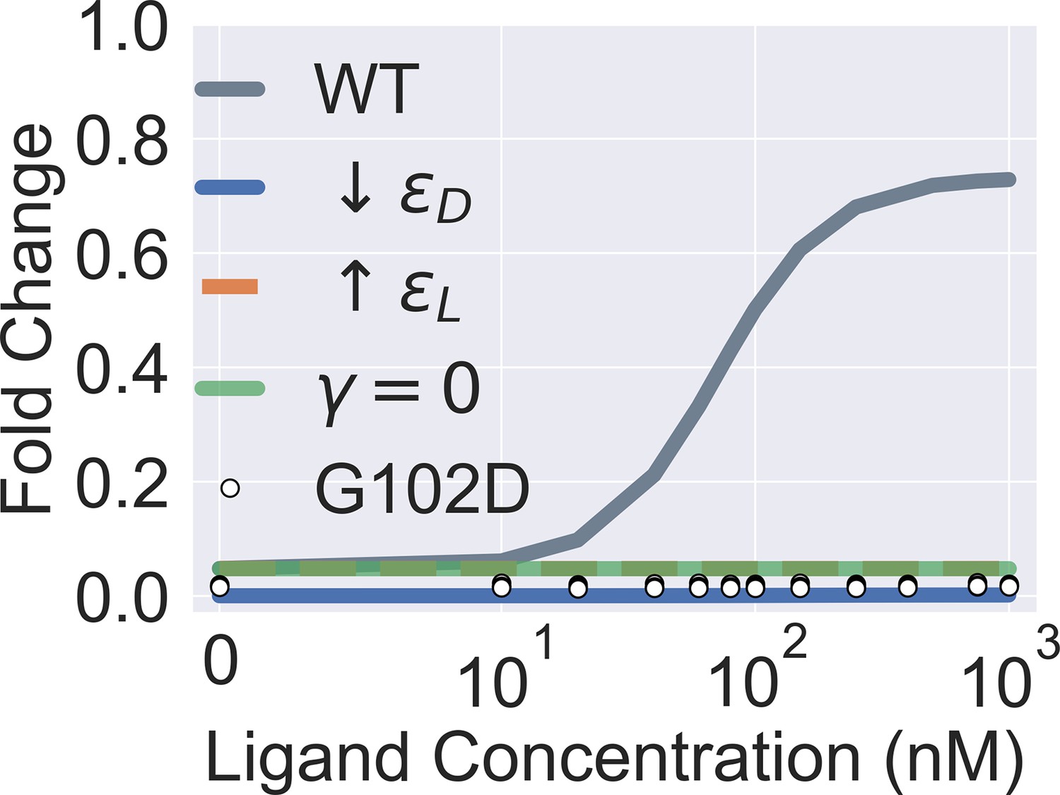
Extended parametric study of main text Equation 1.

The four colored curves show that a flat induction curve can result from tuning each one of the three main biophysical parameters of the two-domain model alone (by decreasing $ε_{D}$ or increasing $ε_{L}$ from the wildtype WT value, or by setting $γ$ to 0). The white points show the experimental induction data for the mutant G102D (measurements of four biological replicates at each ligand concentration). Note that the colored curves in the figure are generated for better visualization of the model parameters’ effect on the induction curve and not to be compared with the experimental data of G102D. The leakiness of G102D (0.0173) is higher than that of the WT (0.0086) determined in experiments.

Figure 3 with 8 supplements

Download asset Open asset

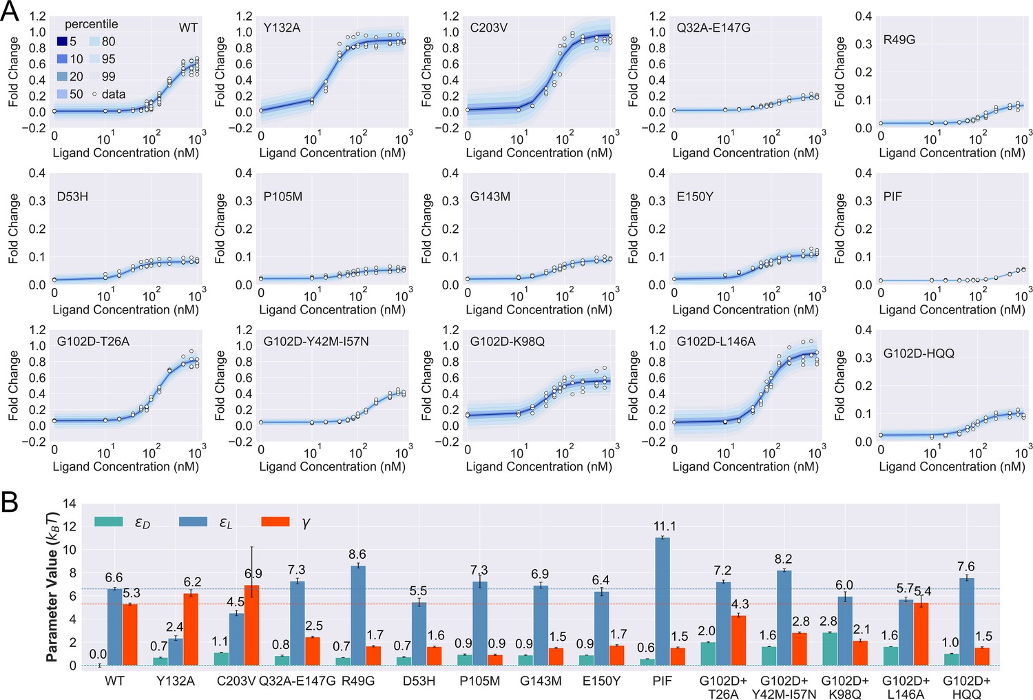
Induction data of 15 TetR mutants and the corresponding parameter estimation results.

(A) Shaded blue curves in each plot show the percentiles of the simulated fold change measurements using the inferred posterior parameters of the mutant. The white data points represent the corresponding experimental induction measurement of four or more biological replicates (three replicates for C203V and G102D-HQQ). (B) The inferred parameter values of the 15 mutants. The error bars of $ε_{L}$ and $γ$ represent the 95th percentile of the Bayesian posterior samples, while the error bar of $ε_{D}$ is calculated based on the standard error of the mean (SEM) of the corresponding leakiness measurement. The horizontal lines indicate the wildtype (WT) parameter values for reference.

Figure 3—figure supplement 1

Download asset Open asset

Sequence and structural distributions of the 21 residues chosen for the mutation analyses in this work.

The upper panel shows the sequence of TetR (residues 2–203), where the 21 residues chosen for mutation analyses in this work are colored red, orange, green, or blue (while the other residues are colored gray). The lower panel shows the crystal structure of TetR(B) in complex with minocycline and magnesium (PDB code: 4AC0). Here, the two identical monomers of TetR are colored white and gray respectively, while the residues chosen for mutation analyses are colored in the same way as in the sequence above in the white monomer. Specifically, the 5 red residues from top to bottom are C203, Y132, I57, R49, and T26. The 4 orange residues from left to right are H44, P105, G102, and L146. The 5 blue residues from top to bottom are Q76, G143, E147, Q47, and Q32. The 7 green residues from left to right are Y42, D53, K98, E150, F177, P176, and I174. Some of the 21 residues are presented in the stick format to aid visualization while all other residues are presented in the cartoon format.

Figure 3—figure supplement 2

Download asset Open asset

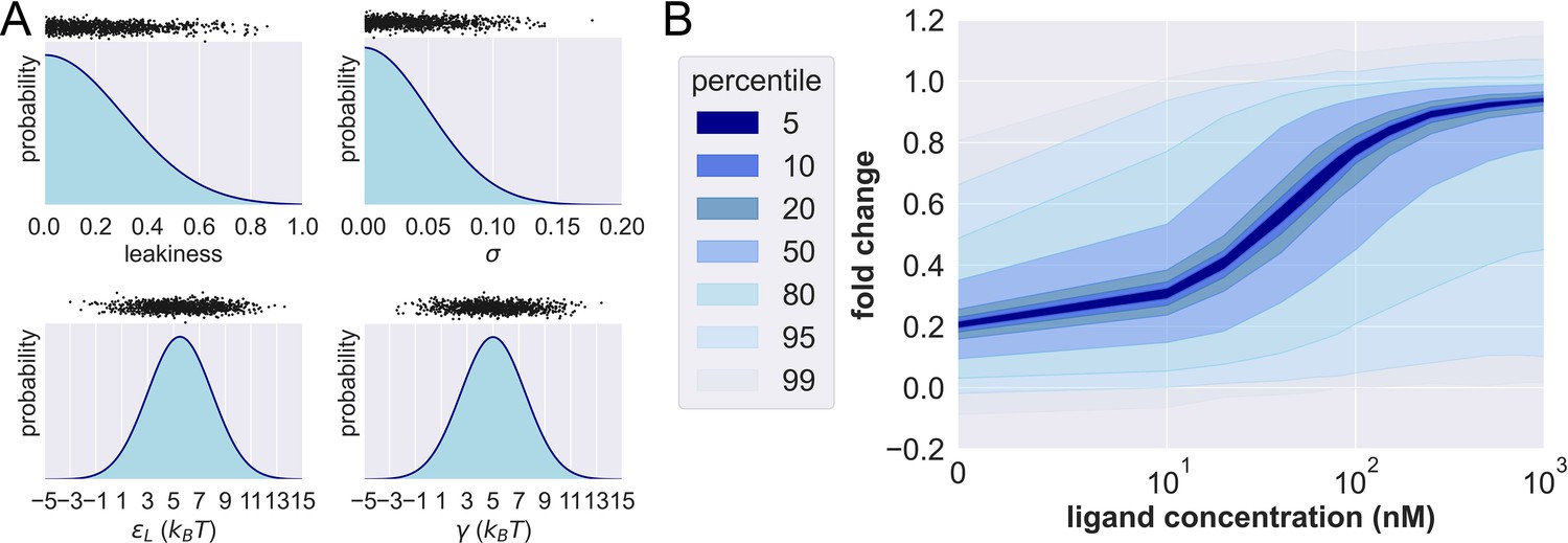
Prior probability distributions and prior predictive check.

(A) Density functions of the prior distributions of leakiness, $σ, ε_{L}, a n d γ$ . The black dots above the prior distributions show the 1000 prior predictive draws of the corresponding parameter. (B) Percentiles of the simulated fold changes using the 1000 sets of parameters shown in (A).

Figure 3—figure supplement 3

Download asset Open asset

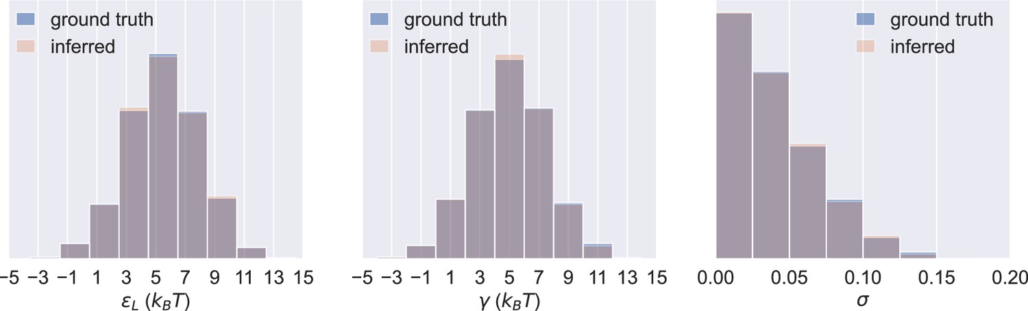
Probability distributions of $ε_{L}, γ, a n d σ$ values in the 1000 sets of prior predictive draws (ground truth) and the average of the corresponding 1000 sets of inferred posterior distributions of the parameters (inferred).

Figure 3—figure supplement 4

Download asset Open asset

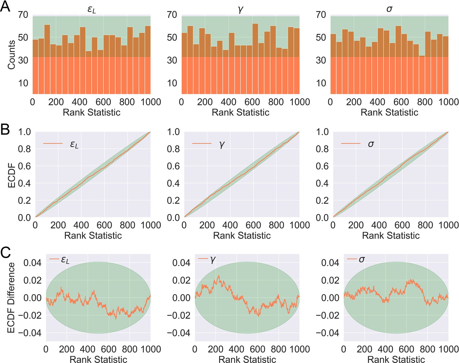
Distributions of rank statistics of the prior predictive draws relative to the corresponding posterior samples.

(A) Histograms (20 bins); (B) ECDF plots; (C) ECDF difference plots of rank statistics of $ε_{L}, γ, a n d σ$ . The green bands in (A)–(C) show the 99th percentile expected from a true uniform distribution.

Figure 3—figure supplement 5

Download asset Open asset

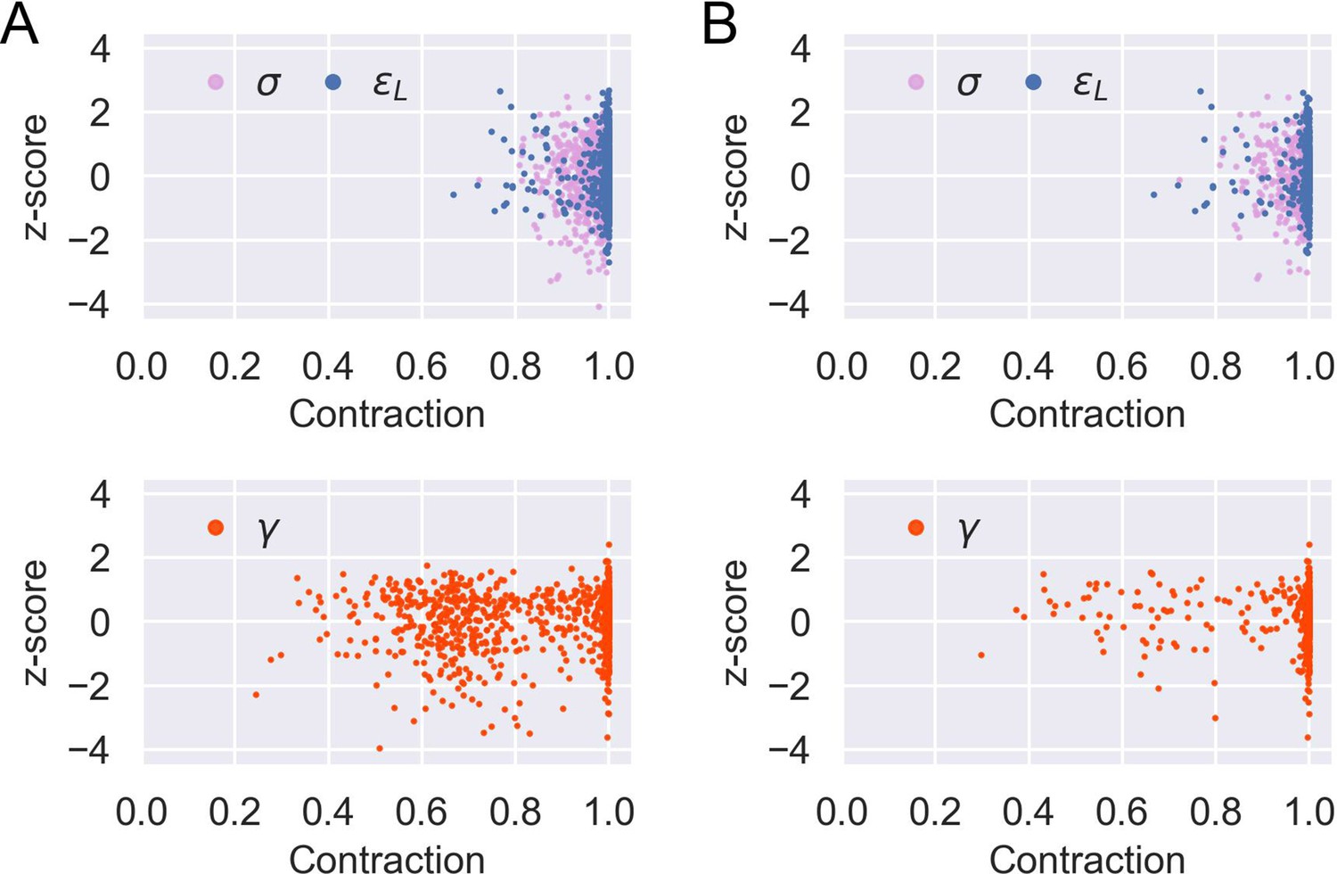
Sensitivity analysis for model parameter inference.

Posterior z-score and posterior contraction of the inferred posterior distribution for each of the 1000 prior predictive draws of parameters and the corresponding simulated data except: (A) parameters of flat induction curves (see Appendix 1 section ‘Model parameter estimation’ and Equation 37); (B) parameters of flat induction curves or $μ (c = 1000 n M) > 0.97$ (see Appendix 1 ‘Model parameter estimation’ and Equation 39). Accordingly, there are 970 and 523 data points for each parameter in (A) and (B), respectively.

Figure 3—figure supplement 6

Download asset Open asset

Posterior predictive check of mutant G102D-Y42M-I57N.

(A) 1000 sets of posterior samples of ${ε_{L}, γ, σ}$ . The scattered plots show the joint distributions of the parameters, colored by the log probability of the parameter combinations. Blue/red corresponds to low/high probability. The histograms show the marginal distributions of the corresponding individual parameters. (B) Percentiles of the simulated fold change measurements using the 1000 sets of posterior samples based on Appendix 1 Equation 29. The white data points show the experimental induction data of four biological replicates.

Figure 3—figure supplement 7

Download asset Open asset

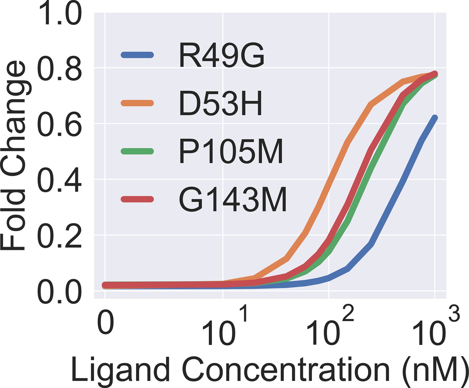
Theoretical induction curves of the four dead mutants when their $γ$ values are set to the wildtype (WT) value while using their respective $ε_{D} a n d ε_{L}$ values (taken from Figure 3B in the main text).

The theoretical induction curve is calculated with main text Equation 1.

Figure 3—figure supplement 8

Download asset Open asset

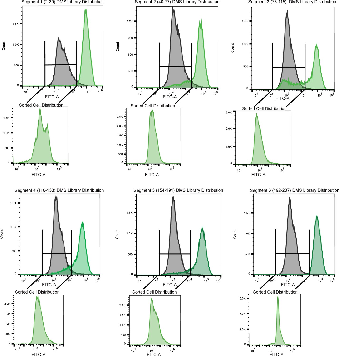
Sorting scheme to identify dead variants.

Each panel is a tiled segment of single site saturation mutants of defined length along the TetR gene. The residue number spanning each segment is shown above the panel. The gray distribution denotes the uninduced population of cells containing mutants. The dark green distribution on the same panel denotes the population of cells responding to the anhydrotetracycline. The uninduced population of cells containing mutants when was added was sorted and reflowed which is shown outside the main panel as the light green distribution.

Figure 4 with 2 supplements

Download asset Open asset

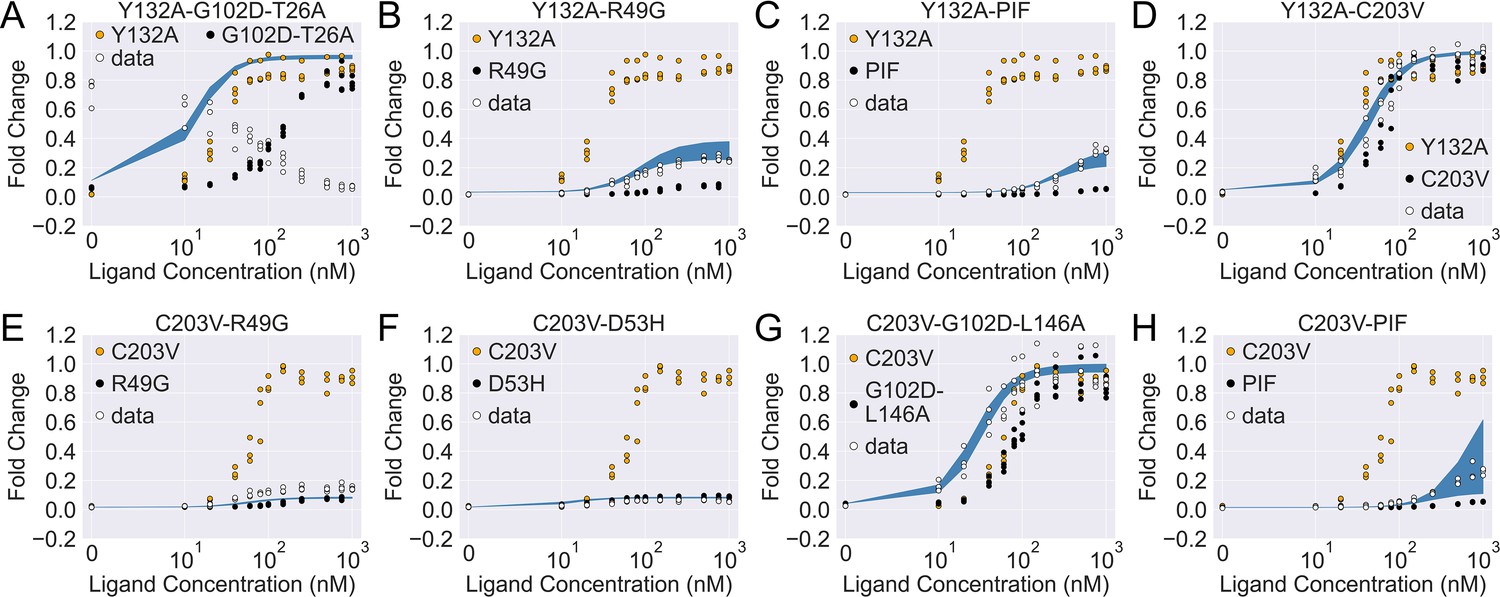
The induction curves for the eight combined TetR mutants from experimental measurement and prediction from the modified additive model.

In each plot, black, orange, and white points represent the experimental data for mutant 1, mutant 2, and the combined mutant (named mutant 1-mutant 2), specified in the legend and title. The blue band shows the 95th percentile of the induction curve prediction from the modified additive model. The modification to the basic additive model in each plot is specified by the six weights ${α_{1, ε_{D}}, α_{2, ε_{D}}, α_{1, ε_{L}}, α_{2, ε_{L}}, α_{1, γ}, α_{2, γ}}$ (see Equation 4), which are (A) ${1, 1, 1, 1, 1, 1}$ ; (B) ${1, 1, 0.5, 1, 1, 1}$ ; (C) ${1, 1, 0.5, 1, 1, 1}$ ; (D) ${1, 1, 0, 1, 1, 1}$ ; (E) ${0, 1, 1, 1, 0, 1}$ ; (F) ${0, 1, 1, 1, 0, 1}$ ; (G) ${0, 1, 1, 1, 1, 1}$ ; (H) ${0, 1, 1, 1, 1, 1}$ .

Figure 4—figure supplement 1

Download asset Open asset

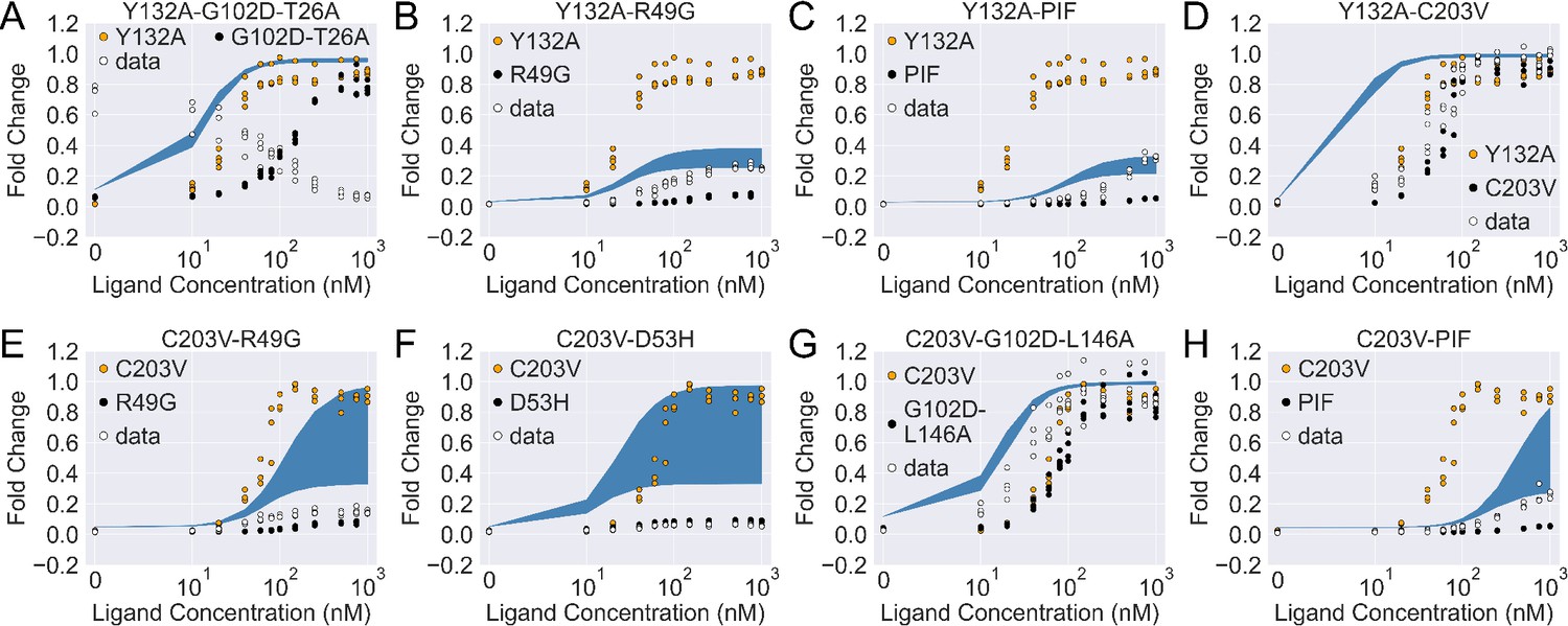
The induction curves of the eight combined mutants calculated using the basic additive model (i.e. with $α_{1, p} = α_{2, p} = 1$ in main text Equation 4).

In each plot, the white data points show the experimental induction data of the combined mutants, while the black and orange ones show data of the individual mutants. The blue band shows the 95th percentile of the induction curve prediction from the additive model.

Figure 4—figure supplement 2

Download asset Open asset

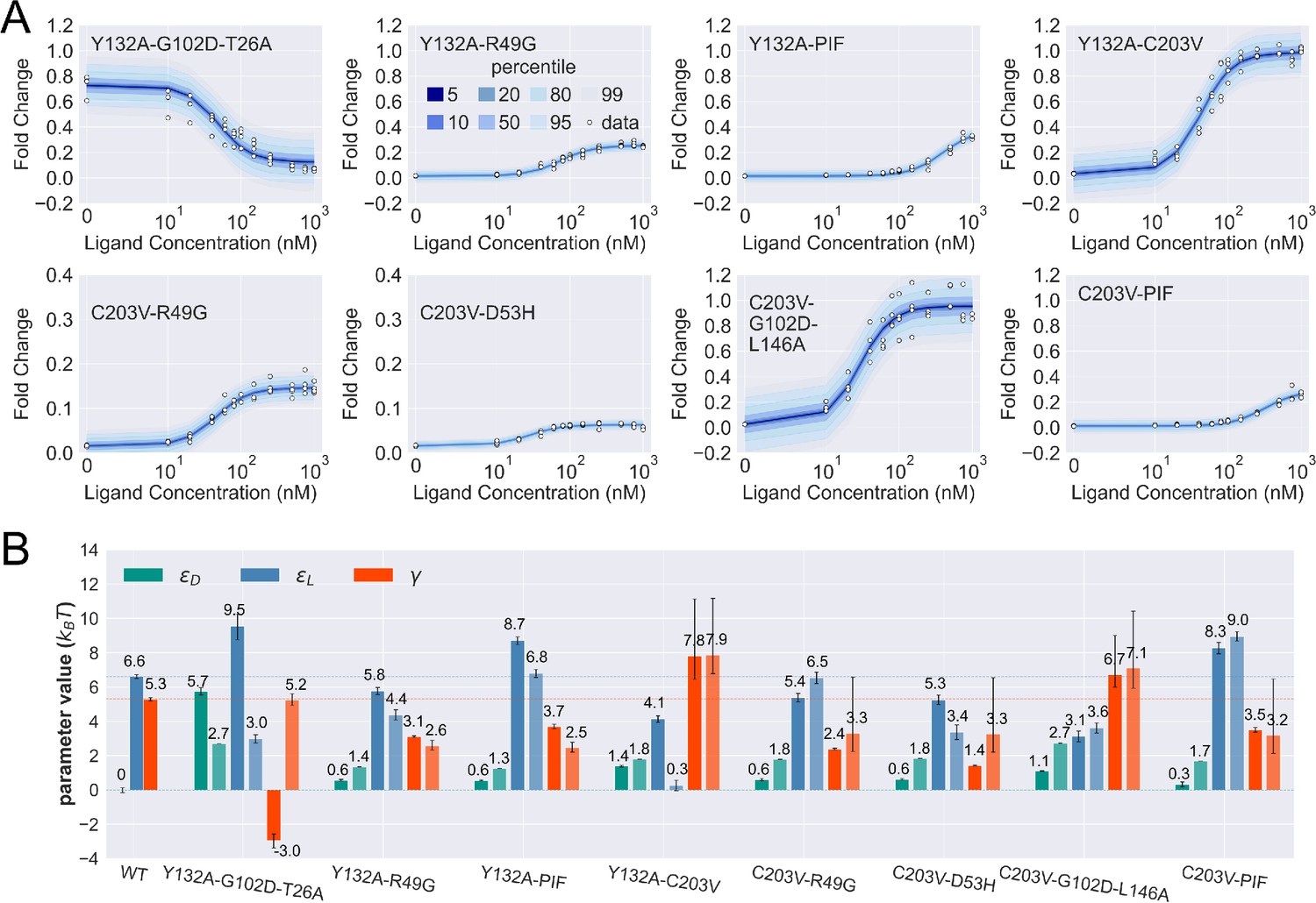
Induction curves of the eight combined mutants and the corresponding parameter estimation results as well as the basic additive model predictions.

(A) Percentiles of the simulated fold change measurements using the inferred posterior parameters of each mutant based on Appendix 1 Equation 29. The white data points show the experimental induction data of four biological replicates (three replicates for C203V-PIF). (B) The inferred parameter values of wildtype (WT) and the eight combined mutants. Error bars of $ε_{L} a n d γ$ represent the upper and lower bounds of the 95% credible region (estimated from 1000 posterior samples). For each combined mutant, the parameters shown by the lighter and darker bar plots are the results from the basic additive model and direct fitting, respectively. The horizontal lines show the WT parameter values for reference. PIF, P176N-I174K-F177S.

Figure 5

Download asset Open asset

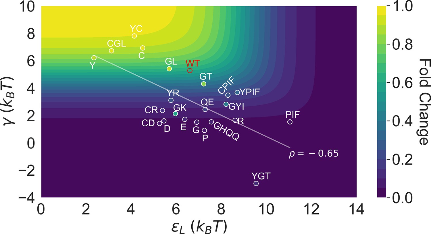
Distribution of the 23 investigated TetR mutants in the parameter space of the two-domain model illustrates the correlation between perturbations in $ε_{L}$ and $γ$ .

Color of the contour plot encodes the fold change at $c = 1000$ nM calculated for each point in the two-dimensional space of $ε_{L}$ and $γ$ with the wildtype (WT) $ε_{D}$ value. The color within the data point of each mutant is based on the $F C^{1000}$ calculated with its specific $ε_{D}$ value. The notation of each mutant is abbreviated based on the one-letter codes of the residues that are mutated. The specific mutations corresponding to each letter code from upper left to lower right are C: C203V; Y: Y132A; GL: G102D-L146A; GT: G102D-T26A; R: R49G; D: D53H; GK: G102D-K98Q; E: E150Y; QE: Q32A-E147G; G: G143M; P: P105M; GYI: G102D-Y42M-I57N; GHQQ: G102D-H44F-Q47S-Q76K; PIF: P176N-I174K-F177S. The least-squares regression line between $ε_{L}$ and $γ$ is shown with their Pearson correlation coefficient ( $ρ$ ).

Tables

Table 1

Distances to the DNA operator and ligand of the 21 residues under mutational study.

Residue number	Distance to DNA operator (Å)	Distance to ligand (Å)
26	7.3	24.7
32	12.6	30.4
42	8.1	25.0
44	9.4	21.6
47	7.7	21.9
49	11.4	17.8
53	17.0	12.1
57	22.5	7.0
76	45.7	17.9
98	19.9	15.6
102	18.1	14.2
105	24.8	7.7
132	39.3	16.0
143	29.4	16.9
146	25.8	17.6
147	26.8	16.0
150	23.2	19.0
174	34.5	14.9
176	38.8	19.5
177	35.5	17.5
203	55.1	28.7

Table 2

Bayesian inference results with different prior distributions of $γ$ .

Mutant	$ϵ_{L}^{1}$	$ϵ_{L}^{2}$	$γ^{1}$	$γ^{2}$
WT	${6.61}_{6.51}^{6.73}$	${6.62}_{6.51}^{6.73}$	${5.29}_{5.20}^{5.38}$	${5.29}_{5.20}^{5.38}$
Q32A-E147G	${7.29}_{7.02}^{7.53}$	${7.27}_{7.02}^{7.53}$	${2.45}_{2.38}^{2.52}$	${2.45}_{2.38}^{2.52}$
R49G	${8.62}_{8.40}^{8.84}$	${8.62}_{8.42}^{8.85}$	${1.66}_{1.60}^{1.72}$	${1.65}_{1.59}^{1.71}$
D53H	${5.46}_{5.09}^{5.80}$	${5.46}_{5.05}^{5.79}$	${1.62}_{1.57}^{1.66}$	${1.62}_{1.57}^{1.67}$
P105M	${7.23}_{6.70}^{7.77}$	${7.24}_{6.59}^{7.76}$	${0.92}_{0.86}^{0.98}$	${0.92}_{0.86}^{0.98}$
Y132A	${2.35}_{2.15}^{2.55}$	${2.36}_{2.17}^{2.55}$	${6.23}_{5.97}^{6.54}$	${6.22}_{5.96}^{6.55}$
G143M	${6.92}_{6.67}^{7.18}$	${6.91}_{6.68}^{7.15}$	${1.52}_{1.47}^{1.56}$	${1.52}_{1.47}^{1.56}$
E150Y	${6.39}_{6.01}^{6.73}$	${6.38}_{5.99}^{6.73}$	${1.72}_{1.66}^{1.79}$	${1.72}_{1.66}^{1.78}$
PIF	${11.05}_{10.92}^{11.17}$	${11.05}_{10.90}^{11.18}$	${1.54}_{1.49}^{1.59}$	${1.54}_{1.49}^{1.59}$
C203V	${4.51}_{4.27}^{4.74}$	${4.53}_{4.27}^{4.78}$	${6.95}_{5.89}^{10.23}$	${7.47}_{6.01}^{15.84}$
G102D-T26A	${7.23}_{7.09}^{7.36}$	${7.22}_{7.11}^{7.35}$	${4.31}_{4.16}^{4.51}$	${4.31}_{4.15}^{4.52}$
G102D-Y42M-I57N	${8.21}_{8.09}^{8.34}$	${8.21}_{8.09}^{8.34}$	${2.83}_{2.78}^{2.89}$	${2.83}_{2.78}^{2.88}$
G102D-K98Q	${5.96}_{5.51}^{6.36}$	${5.97}_{5.55}^{6.37}$	${2.14}_{2.01}^{2.28}$	${2.14}_{2.00}^{2.29}$
G102D-L146A	${5.70}_{5.51}^{5.88}$	${5.70}_{5.52}^{5.88}$	${5.43}_{5.03}^{6.05}$	${5.42}_{5.03}^{6.05}$
G102D-HQQ	${7.56}_{7.30}^{7.83}$	${7.57}_{7.23}^{7.86}$	${1.54}_{1.48}^{1.61}$	${1.54}_{1.48}^{1.60}$
Y132A-G102D-T26A	${9.55}_{8.77}^{10.25}$	${9.67}_{8.92}^{10.51}$	$- {2.96}_{- 3.39}^{- 2.58}$	$- {3.02}_{- 3.47}^{- 2.66}$
Y132A-R49G	${5.77}_{5.56}^{5.98}$	${5.78}_{5.58}^{5.98}$	${3.11}_{3.05}^{3.16}$	${3.11}_{3.05}^{3.16}$
Y132A-PIF	${8.71}_{8.48}^{8.93}$	${8.70}_{8.47}^{8.93}$	${3.69}_{3.57}^{3.84}$	${3.69}_{3.57}^{3.83}$
Y132A-C203V	${4.14}_{3.94}^{4.32}$	${4.15}_{3.96}^{4.34}$	${7.82}_{6.46}^{11.12}$	${9.30}_{6.76}^{16.72}$
C203V-R49G	${5.40}_{5.14}^{5.63}$	${5.39}_{5.13}^{5.66}$	${2.38}_{2.33}^{2.43}$	${2.38}_{2.33}^{2.44}$
C203V-D53H	${5.26}_{4.98}^{5.53}$	${5.26}_{4.97}^{5.51}$	${1.42}_{1.39}^{1.46}$	${1.43}_{1.39}^{1.46}$
C203V-G102D-L146A	${3.13}_{2.81}^{3.43}$	${3.16}_{2.78}^{3.49}$	${6.74}_{6.00}^{9.01}$	${6.99}_{6.03}^{13.63}$
C203V-PIF	${8.30}_{7.95}^{8.61}$	${8.30}_{7.94}^{8.65}$	${3.49}_{3.36}^{3.64}$	${3.49}_{3.35}^{3.64}$

The column of $p^{1} / p^{2}$ shows the Bayesian inference results using the Gaussian prior distribution of $γ$ centered at 5 $k_{B} T$ with a standard deviation of 2.5/5 $k_{B} T (p = ϵ_{L} o r γ)$ . The numbers in the table are the medians of the inferred posterior distributions for the corresponding parameters, with their superscripts/subscripts labeling the upper/lower bound of the 95% credible regions (estimated from 1000 posterior samples).

Additional files

MDAR checklist: https://cdn.elifesciences.org/articles/92262/elife-92262-mdarchecklist1-v1.docx
Download elife-92262-mdarchecklist1-v1.docx

Download links

A two-part list of links to download the article, or parts of the article, in various formats.

Downloads (link to download the article as PDF)

Open citations (links to open the citations from this article in various online reference manager services)

Mendeley

Cite this article (links to download the citations from this article in formats compatible with various reference manager tools)

Zhuang Liu
Thomas G Gillis
Srivatsan Raman
Qiang Cui

(2024)

A parameterized two-domain thermodynamic model explains diverse mutational effects on protein allostery

eLife 12:RP92262.

https://doi.org/10.7554/eLife.92262.3

Share this article

Cite this article

Schematic illustration of the two-domain statistical thermodynamic model of TetR allostery.

Schematic illustration of the characteristic effects of perturbations in the three biophysical parameters on the free energy landscape and the corresponding induction curves of a two-domain allosteric system.

Statistical weights of promoter occupancy states and repressor states.

Equilibria among different conformational and binding states of the repressor.

Extended parametric study of main text Equation 1.

Induction data of 15 TetR mutants and the corresponding parameter estimation results.

Sequence and structural distributions of the 21 residues chosen for the mutation analyses in this work.

Prior probability distributions and prior predictive check.

Probability distributions of εL,γ,andσ values in the 1000 sets of prior predictive draws (ground truth) and the average of the corresponding 1000 sets of inferred posterior distributions of the parameters (inferred).

Distributions of rank statistics of the prior predictive draws relative to the corresponding posterior samples.

Sensitivity analysis for model parameter inference.

Posterior predictive check of mutant G102D-Y42M-I57N.

Theoretical induction curves of the four dead mutants when their γ values are set to the wildtype (WT) value while using their respective εDandεL values (taken from Figure 3B in the main text).

Sorting scheme to identify dead variants.

The induction curves for the eight combined TetR mutants from experimental measurement and prediction from the modified additive model.

The induction curves of the eight combined mutants calculated using the basic additive model (i.e. with α1,p=α2,p=1 in main text Equation 4).

Induction curves of the eight combined mutants and the corresponding parameter estimation results as well as the basic additive model predictions.

Distribution of the 23 investigated TetR mutants in the parameter space of the two-domain model illustrates the correlation between perturbations in εL and γ.

Distances to the DNA operator and ligand of the 21 residues under mutational study.

Bayesian inference results with different prior distributions of γ.

MDAR checklist

Downloads (link to download the article as PDF)

Open citations (links to open the citations from this article in various online reference manager services)

Cite this article (links to download the citations from this article in formats compatible with various reference manager tools)

Probability distributions of $ε_{L}, γ, a n d σ$ values in the 1000 sets of prior predictive draws (ground truth) and the average of the corresponding 1000 sets of inferred posterior distributions of the parameters (inferred).

Theoretical induction curves of the four dead mutants when their $γ$ values are set to the wildtype (WT) value while using their respective $ε_{D} a n d ε_{L}$ values (taken from Figure 3B in the main text).

The induction curves of the eight combined mutants calculated using the basic additive model (i.e. with $α_{1, p} = α_{2, p} = 1$ in main text Equation 4).

Distribution of the 23 investigated TetR mutants in the parameter space of the two-domain model illustrates the correlation between perturbations in $ε_{L}$ and $γ$ .

Bayesian inference results with different prior distributions of $γ$ .