The neural correlates of novelty and variability in human decision-making under an active inference framework
- Centre for Cognitive and Brain Sciences and Department of Psychology, University of Macau, China
- Department of Biomedical Engineering, Southern University of Science and Technology, China
Figures
Figure 1
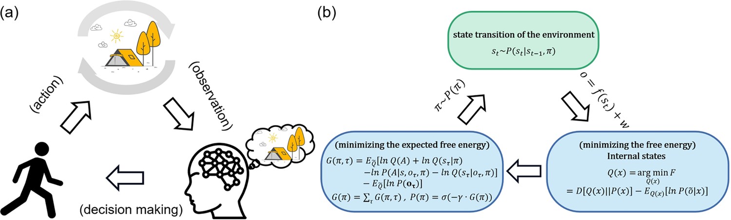
Active inference.
(a) Qualitatively, agents receive observations from the environment and use these observations to optimize Bayesian beliefs under an internal cognitive (a.k.a., world or generative) model of the environment. Then agents actively sample the environment states by action, choosing actions that would make them in more favorable states. The environment changes its state according to agents’ policies (action sequences) and transition functions. Then again, agents receive new observations from the environment. (b) From a quantitative perspective, agents optimize the Bayesian beliefs under an internal cognitive (a.k.a., world or generative) model of the environment by minimizing the variational free energy. Then agents select policies minimizing the expected free energy, namely, the surprise expected in the future under a particular policy.
Figure 2
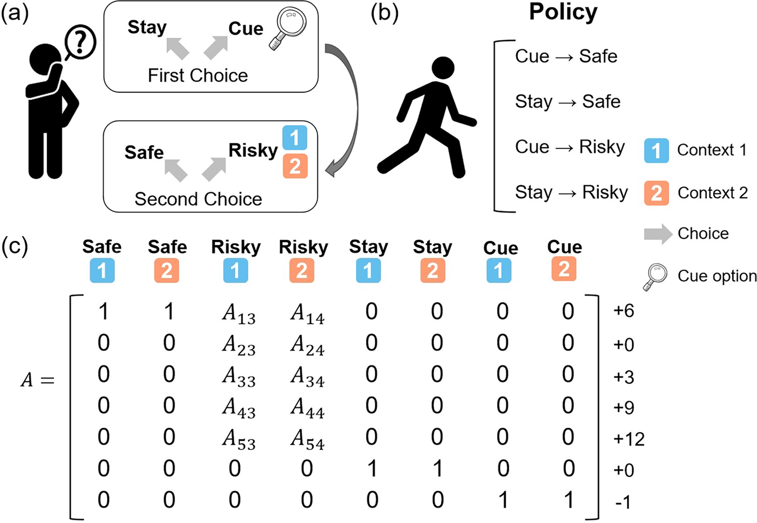
The contextual two-armed bandit task.
(a) In this task, agents need to make two choices in each trial. The first choice is “Stay” and “Cue”. The “Stay” option gives you nothing while the “Cue” option gives you a –1 reward and the context information about the “Risky” option in the current trial. The second choice is “Safe” and “Risky”. The “Safe” option always gives you a +6 reward and the “Risky” option gives you a reward probabilistically, ranging from 0 to +12 depending on the current context (context 1 or context 2). (b) The four policies in this task are “Cue” and “Safe”, “Stay” and “Safe”, “Cue” and “Risky”, and “Stay” and “Risky”. (c) The likelihood matrix maps from 8 hidden states (columns) to 7 observations (rows).
Figure 3
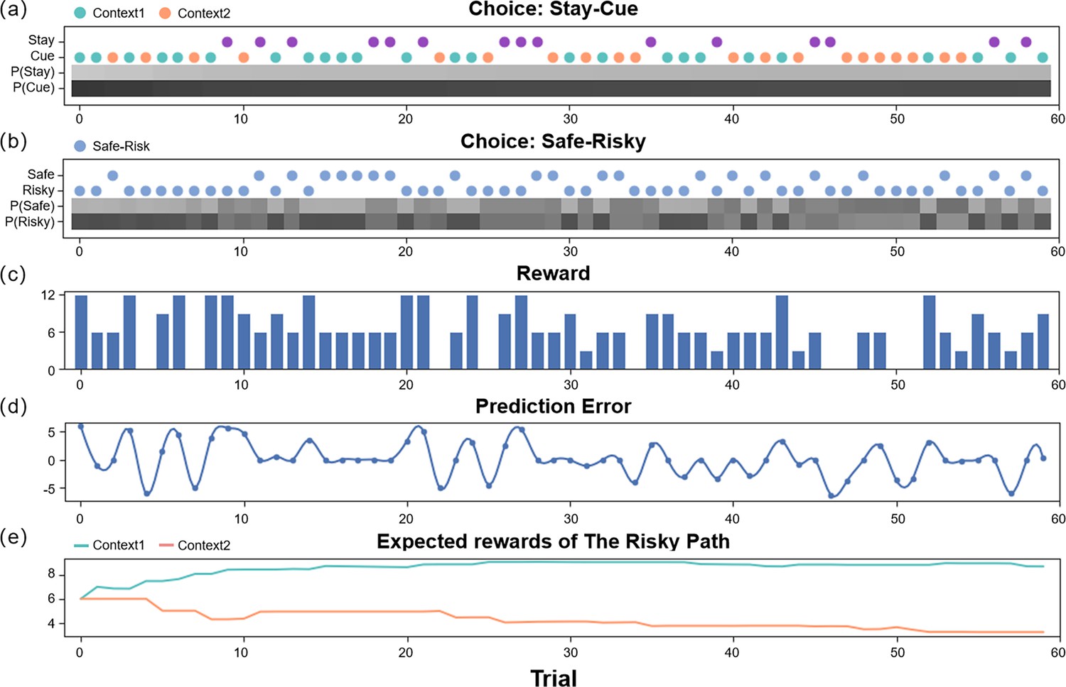
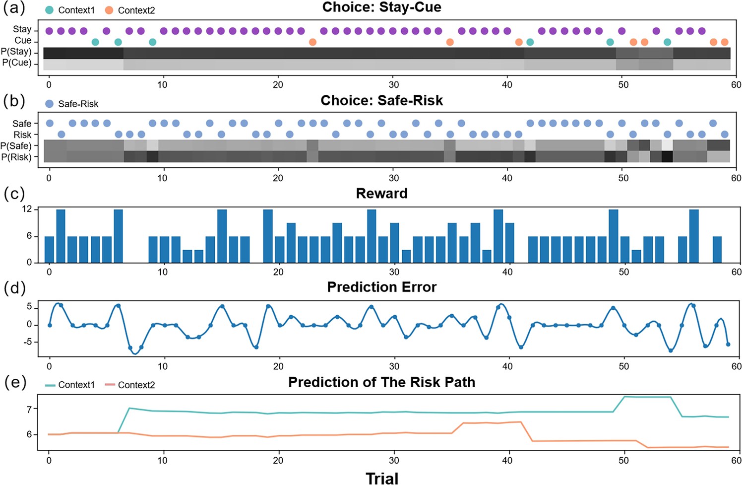
The simulation experiment results.
This figure demonstrates how an agent selects actions and updates beliefs over 60 trials in the active inference framework. The first two panels (a, b) display the agent’s policy and depict how the policy probabilities are updated (choosing between the stay or cue option in the first choice, and selecting between the safe or risky option in the second choice). The scatter plot indicates the agent’s actions, with green representing the cue option when the context of the risky path is “Context 1” (high-reward context), orange representing the cue option when the context of the risky path is “Context 2” (low-reward context), purple representing the stay option when the agent is uncertain about the context of the risky path, and blue indicating the safe-risky choice. The shaded region represents the agent’s confidence, with darker shaded regions indicating greater confidence. The third panel (c) displays the rewards obtained by the agent in each trial. The fourth panel (d) shows the prediction error of the agent in each trial, which decreases over time. Finally, the fifth panel (e) illustrates the expected rewards of the ‘Risky Path’ in the two contexts of the agent.
Figure 4
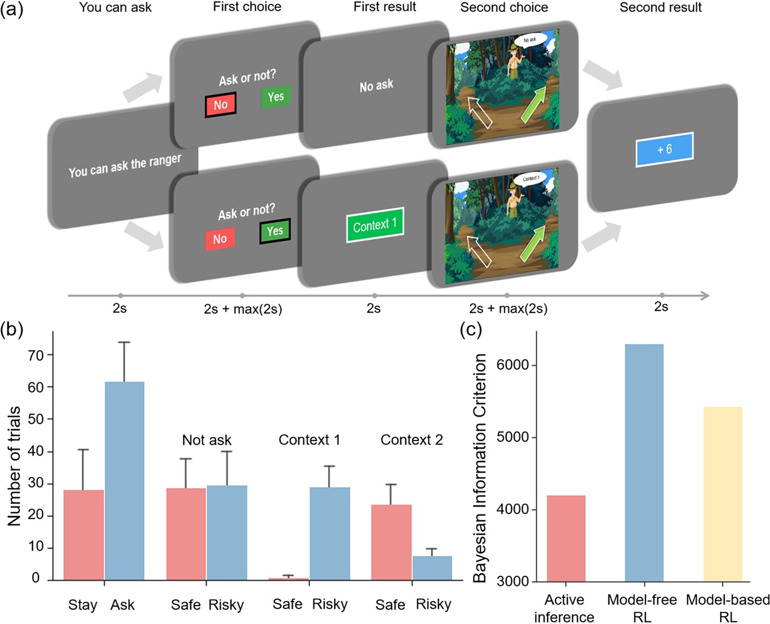
The experiment task and behavioral result.
(a) The five stages of the experiment, which include the “You can ask” stage to prompt the participants to decide whether to request information from the Ranger, the “First choice” stage to decide whether to ask the ranger for information, the “First result” stage to display the result of the “First choice” stage, the “Second choice” stage to choose between left and right paths under different uncertainties and the “Second result” stage to show the result of the “Second choice” stage. The error bars show the 95% confidence interval. (b) The number of times each option was selected. The error bar indicates the variance among participants. (c) The Bayesian information criterion of active inference, model-free reinforcement learning, and model-based reinforcement learning.
Figure 5
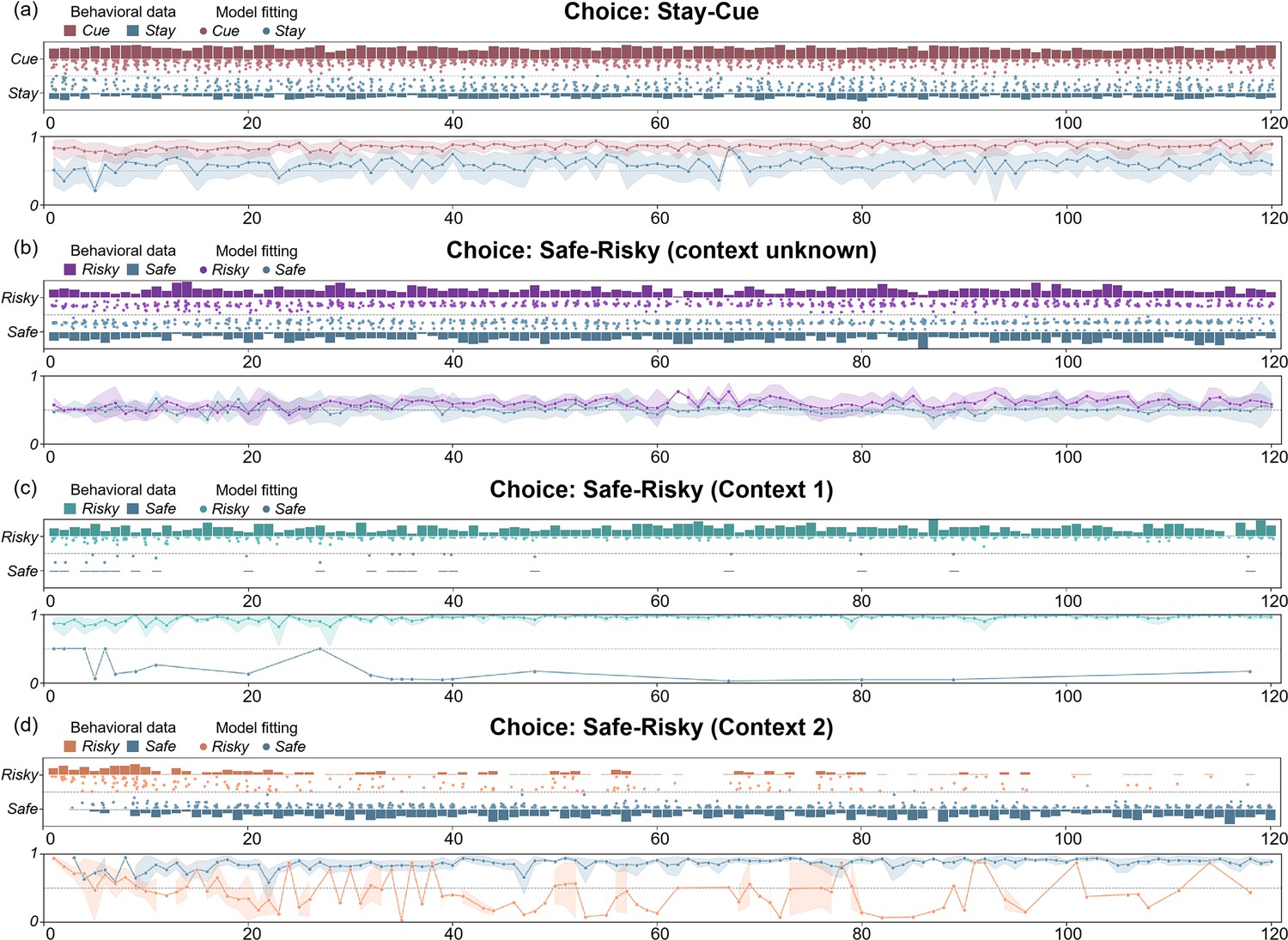
The comparison between the active inference model and the behavioral data in (a) the “First choice” stage, and the “Second choice” stage; (b) context unknown, (c) “Context 1”, and (d) “Context 2”.
The bar graphs show participants’ behavior data in each trial, and the height shows the proportion of participants who chose a certain option in each trial. The scatter plots show the model’s fitting results for the two choices of the participants. The closer the point is to the bar graph on both sides, the higher the fitting accuracy. The line graphs show the trend of the model fitting accuracies with the trials.
Figure 6
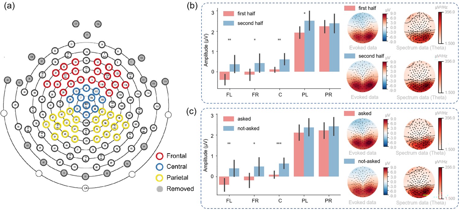
EEG results at the sensor level.
(a) The electrode distribution. (b) The signal amplitude of different brain regions in the first and second half of the experiment in the “Second choice” stage. The error bar indicates the amplitude variance in each region. The right panel shows the visualization of the evoked data and spectrum data. (c) The signal amplitude of different brain areas in the “Second choice” stage where participants know the context or do not know the context of the right path. The error bar indicates the amplitude variance in each region. The error bars show the 95% confidence interval. The right panel shows the visualization of the evoked data and spectrum data. FL: frontal-left; FR: frontal-right; C: central; PL: parietal-left; PR: parietal-right.
Figure 7
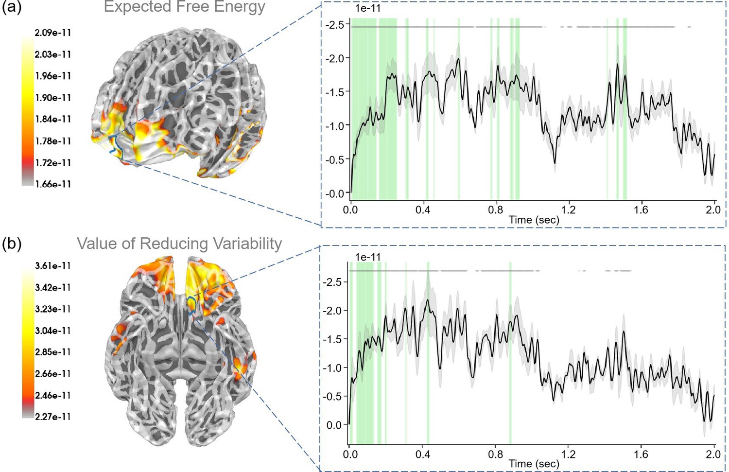
The source estimation results of expected free energy and active inference in the “First choice” stage.
(a) The regression intensity () of expected free energy. The right panel indicates the regression intensity between the frontal pole (1, right half) and the expected free energy. The green-shaded regions indicate p<0.05 after false discovery rate (FDR) correction (the average t-value during these significant periods equals −3.228). (b) The regression intensity () of the value of reducing variability. The right panel indicates the regression intensity between the medial orbitofrontal cortex (5, left half) and the value of reducing variability. The green-shaded regions indicate p<0.05 after FDR correction (the average t-value during these significant periods equals −3.081). The black lines indicate the average intensities, and the gray-shaded regions indicate the ranges of variations (the 95% confidence interval). The gray lines indicate p<0.05 before FDR.
Figure 8
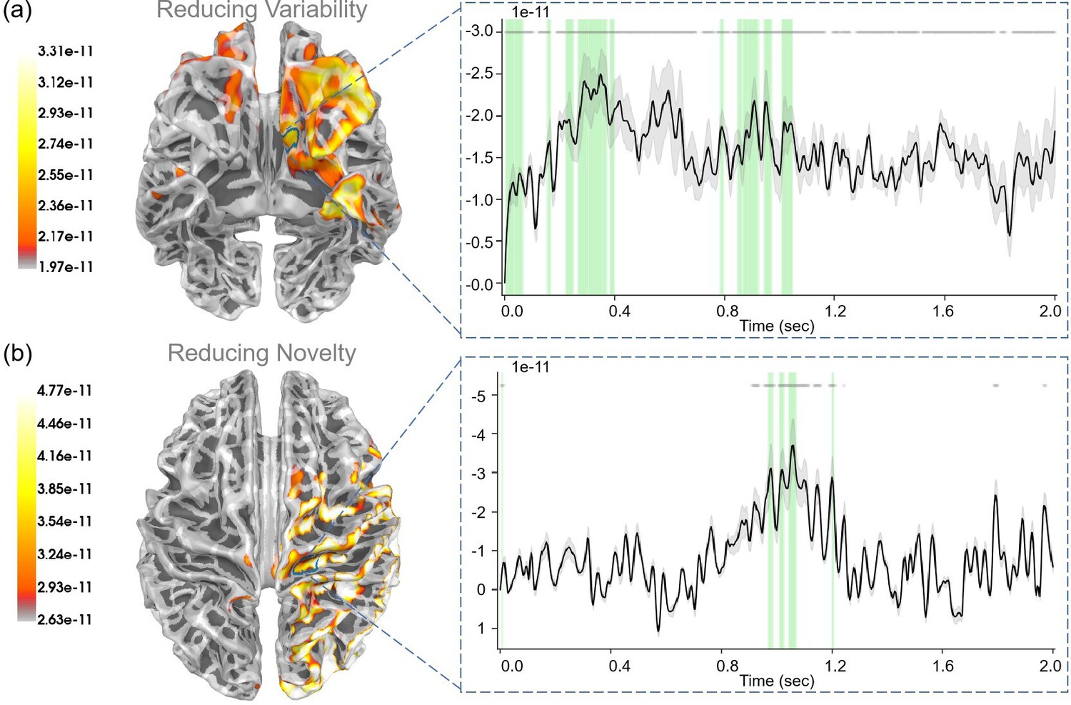
The source estimation results of reducing variability and reducing novelty in the two result stages.
(a) The regression intensity (β) of reducing variability in the “First result” stage. The right panel indicates the regression intensity between the medial orbitofrontal cortex (5, left half) and reducing variability. The green-shaded regions indicate p<0.05 after false discovery rate (FDR) correction (the average t-value during these significant periods equals −3.001). (b) The regression intensity () of reducing novelty in the “Second result” stage. The right panel indicates the regression intensity between the precentral gyrus (15, right half) and reducing novelty. The green-shaded regions indicate p<0.05 after FDR correction (the average t-value during these significant periods equals ). The black lines indicate the average intensities, and the gray-shaded regions indicate the ranges of variations (the 95% confidence interval). The gray lines indicate p<0.05 before FDR.
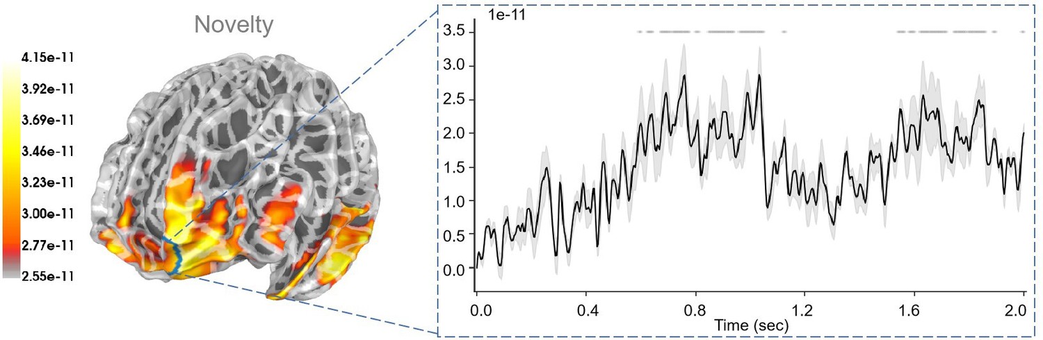
Figure 9
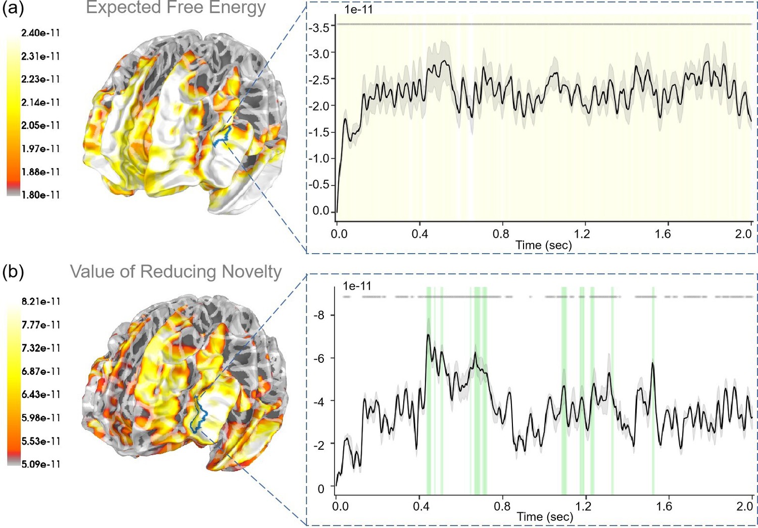
The source estimation results of expected free energy and the value of reducing novelty in the “Second choice” stage.
(a) The regression intensity () of expected free energy. The right panel indicates the regression intensity between the rostral middle frontal gyrus (1, left half) and expected free energy, the black line indicates the average intensity of this region, and the gray-shaded region indicates the range of variation. The yellow-shaded regions indicate p<0.001 after false discovery rate (FDR) (the average t-value during these significant periods equals −4.819) and the gray lines indicate p<0.001 before FDR. (b) The regression intensity (β) of the value of reducing novelty. The right panel indicates the regression intensity between the rostral middle frontal gyrus (6, left half) and the value of reducing novelty, the black line indicates the average intensity of this region, and the gray-shaded region indicates the range of variation (the 95% confidence interval). The green-shaded regions indicate p<0.05 after FDR (the average t-value during these significant periods equals −3.067) and the gray lines indicate p<0.05 before FDR.
Appendix 1—figure 1

The simulation experiment results.
This figure demonstrates how an agent selects actions and updates beliefs over 60 trials in the active inference framework. The first two panels (a, b) display the agent’s policy and depict how the policy probabilities are updated (choosing between the stay or cue option in the first choice, and selecting between the safe or risky option in the second choice). The scatter plot indicates the agent’s actions, with green representing the cue option when the context of the risky path is “Context 1” (high-reward context), orange representing the cue option when the context of the risky path is “Context 2” (low-reward context), purple representing the stay option when the agent is uncertain about the context of the risky path, and blue indicating the safe-risky choice. The shaded region represents the agent’s confidence, with darker shaded regions indicating greater confidence. The third panel (c) displays the rewards obtained by the agent in each trial. The fourth panel (d) shows the prediction error of the agent in each trial. Finally, the fifth panel (e) illustrates the expected rewards of the “Risky Path” in the two contexts of the agent.
Appendix 1—figure 2
The simulation experiment results.
This figure demonstrates how an agent selects actions and updates beliefs over 60 trials in the active inference framework. The first two panels (a, b) display the agent’s policy and depict how the policy probabilities are updated (choosing between the stay or cue option in the first choice, and selecting between the safe or risky option in the second choice). The scatter plot indicates the agent’s actions, with green representing the cue option when the context of the risky path is “Context 1” (high-reward context), orange representing the cue option when the context of the risky path is “Context 2” (low-reward context), purple representing the stay option when the agent is uncertain about the context of the risky path, and blue indicating the safe-risky choice. The shaded region represents the agent’s confidence, with darker shaded regions indicating greater confidence. The third panel (c) displays the rewards obtained by the agent in each trial. The fourth panel (d) shows the prediction error of the agent in each trial. Finally, the fifth panel (e) illustrates the expected rewards of the “Risky Path” in the two contexts of the agent.
Appendix 1—figure 3
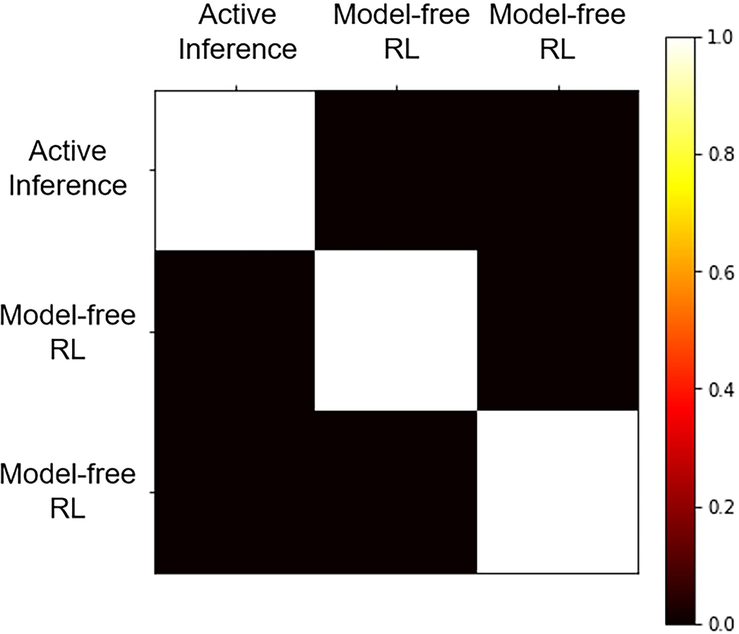
Model recovery results.
Appendix 1—figure 4
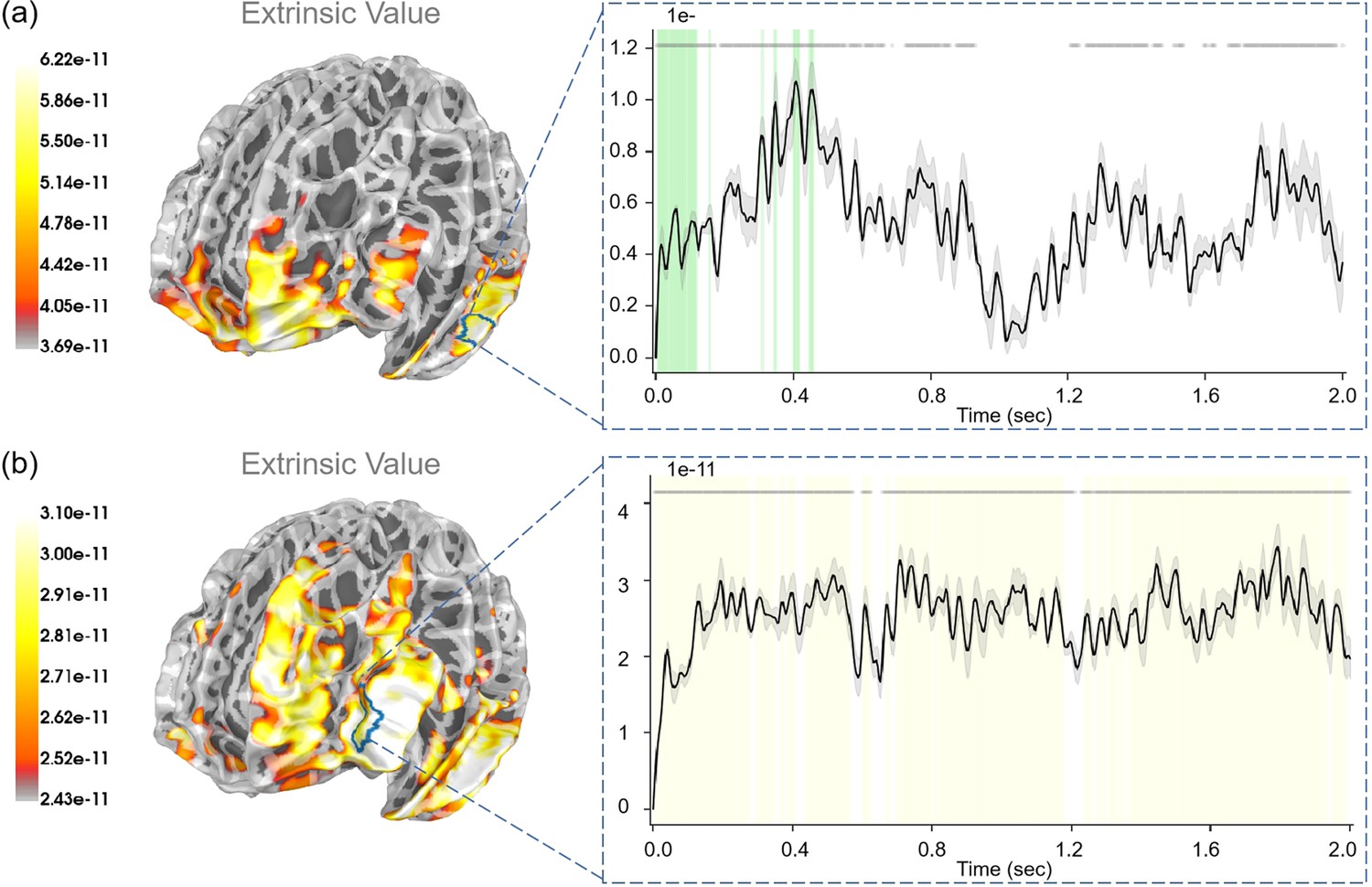
The source estimation results of extrinsic value in the two choosing stages.
(a) The regression intensity () of extrinsic value in the “First choice” stage. The right panel indicates the regression intensity between the middle temporal gyrus (6, right half) and extrinsic value. The green-shaded regions indicate p<0.05 after false discovery rate (FDR) correction (the average t-value during these significant periods equals 3.673). (b) The regression intensity () of extrinsic value in the “Second choice” stage. The right panel indicates the regression intensity between the rostral middle frontal gyrus (6, left half) and extrinsic value. The yellow-shaded regions indicate p<0.001 after FDR correction (the average t-value during these significant periods equals ). The black lines indicate the average intensities, and the gray-shaded regions indicate the ranges of variations. The gray lines indicate p<0.05 before FDR.
Appendix 1—figure 5
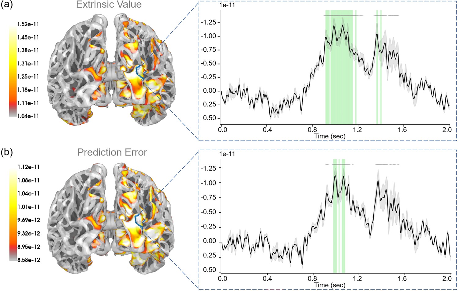
The source estimation results of extrinsic value and prediction error in the “Second result” stage.
(a) The regression intensity () of extrinsic value. The right panel indicates the regression intensity between the lateral occipital cortex (3, right half) and extrinsic value. The green-shaded regions indicate p<0.05 after false discovery rate (FDR) correction (the average t-value during these significant periods equals 2.875). (b) The regression intensity () of prediction error. The right panel indicates the regression intensity between the lateral occipital cortex (3, right half) and prediction error. The green-shaded regions indicate p<0.05 after FDR correction (the average t-value during these significant periods equals –2.716). The black lines indicate the average intensities, and the gray-shaded regions indicate the ranges of variations. The gray lines indicate p<0.05 before FDR.
Appendix 1—figure 6
The source estimation results of ambiguity in the “Second choice” stage.
The right panel indicates the regression intensity between the frontal pole (1, left half) and ambiguity. The black line indicates the average intensities, and the gray-shaded regions indicate the ranges of variations. The gray lines indicate p<0.05 before FDR.
Tables
Table 1
Ingredients for computational modeling of active inference.
| Notations | Definition | Description |
|---|---|---|
| O | A finite set of observations (outcomes) | Sensory input that brains receive. |
| S | A finite set of hidden states | The true hidden states of the environment that generate sensory inputs to brains. |
| U | A finite set of actions | Agent performs actions that change the environment. |
| T | A finite set of time-sensitive policies | A policy is an action sequence over time. |
| R | A generative process | The generative process generates observations and next states (state transitions of the environment) based on current states and actions. |
| P | A generative model | The generative model describes what the agent believes about the environment (how observations are generated). |
| Q | An approximate posterior | The Bayesian beliefs under the generative model that is optimized to minimize variational free energy. By definition, these beliefs correspond to approximate posteriors. |
Appendix 1—table 1
In the “Stay/Cue” choice, we require that the activity of more than 50% of brain regions remains significantly correlated with the expected free energy for over 0.32 seconds, with a significance p<0.05 (after false discovery rate correction).
The brain regions are delineated according to the "aparc sub" parcellation.
| Regressor | p-Value | Proportion | Duration | |
|---|---|---|---|---|
| Expected free energy | 0.01 | 0.5 | 0.32 seconds | |
| Brain region | Duration | Proportion | Regression coefficient | t-Value |
| Frontalpole 1-lh | 0.34 | 0.8965 | 1.342 × 10⁻¹¹ | –3.136 |
| Frontalpole 1-rh | 0.372 | 0.9086 | 1.357 × 10⁻¹¹ | –3.228 |
| Lateralorbitofrontal 2-lh | 0.364 | 0.8608 | 1.526 × 10⁻¹¹ | –3.235 |
| Lateralorbitofrontal 3-lh | 0.332 | 0.7691 | 1.362 × 10⁻¹¹ | –3.195 |
| Lateralorbitofrontal 5-lh | 0.336 | 0.7778 | 1.365 × 10⁻¹¹ | –3.126 |
| Lateralorbitofrontal 5-rh | 0.332 | 0.8193 | 1.333 × 10⁻¹¹ | –2.984 |
| Lateralorbitofrontal 6-lh | 0.372 | 0.9086 | 1.550 × 10⁻¹¹ | –3.335 |
| Lateralorbitofrontal 7-lh | 0.332 | 0.8614 | 1.584 × 10⁻¹¹ | –3.062 |
| Lateralorbitofrontal 7-rh | 0.34 | 0.8902 | 1.530 × 10⁻¹¹ | –3.059 |
| Medialorbitofrontal 1-lh | 0.356 | 0.9711 | 1.624 × 10⁻¹¹ | –3.068 |
| Medialorbitofrontal 1-rh | 0.348 | 0.9234 | 1.563 × 10⁻¹¹ | –3.049 |
| Medialorbitofrontal 2-lh | 0.348 | 0.9163 | 1.360 × 10⁻¹¹ | –3.038 |
| Medialorbitofrontal 3-rh | 0.336 | 0.9048 | 1.402 × 10⁻¹¹ | –3.016 |
| Medialorbitofrontal 4-lh | 0.364 | 0.8767 | 1.436 × 10⁻¹¹ | –3.165 |
| Medialorbitofrontal 5-lh | 0.38 | 0.8579 | 1.502 × 10⁻¹¹ | –3.420 |
| Rostralmiddlefrontal 11-lh | 0.364 | 0.8773 | 1.604 × 10⁻¹¹ | –3.200 |
| Rostralmiddlefrontal 11-rh | 0.344 | 0.8469 | 1.486 × 10⁻¹¹ | –3.112 |
| Rostralmiddlefrontal 12-lh | 0.344 | 0.8857 | 1.494 × 10⁻¹¹ | –3.120 |
| Rostralmiddlefrontal 12-rh | 0.336 | 0.7840 | 1.189 × 10⁻¹¹ | –3.210 |
| Rostralmiddlefrontal 13-rh | 0.34 | 0.8510 | 1.428 × 10⁻¹¹ | –3.220 |
| Superiorfrontal 1-lh | 0.336 | 0.9122 | 1.420 × 10⁻¹¹ | –3.101 |
Appendix 1—table 2
In the “Stay/Cue” choice, we require that the activity of more than 50% of brain regions remains significantly correlated with the value of reducing risk for over 0.152 seconds, with a significance p<0.05 (after false discovery rate correction).
The brain regions are delineated according to the "aparc sub" parcellation.
| Regressor | p-Value | Proportion | Duration | |
|---|---|---|---|---|
| Value of avoiding risk | 0.05 | 0.5 | 0.152 seconds | |
| Brain region | Duration | Proportion | Regression coefficient | t-Value |
| Caudalmiddlefrontal 5-lh | 0.152 | 0.9676 | 1.151 × 10⁻¹¹ | –3.363 |
| Caudalmiddlefrontal 6-lh | 0.156 | 0.9837 | 1.006 × 10⁻¹¹ | –3.307 |
| Insula 2-lh | 0.156 | 0.9597 | 1.270 × 10⁻¹¹ | –3.350 |
| Insula 3-lh | 0.156 | 0.9359 | 1.229 × 10⁻¹¹ | –3.251 |
| Medialorbitofrontal 5-lh | 0.164 | 0.8659 | 1.386 × 10⁻¹¹ | –3.081 |
| Parsopercularis 3-lh | 0.160 | 0.9479 | 1.450 × 10⁻¹¹ | –3.334 |
| Postcentral 10-lh | 0.160 | 0.9450 | 1.071 × 10⁻¹¹ | –3.054 |
| Postcentral 11-lh | 0.152 | 0.9737 | 1.111 × 10⁻¹¹ | –3.171 |
| Postcentral 13-lh | 0.152 | 0.8991 | 1.190 × 10⁻¹¹ | –2.951 |
| Precentral 11-lh | 0.152 | 0.9799 | 1.033 × 10⁻¹¹ | –3.376 |
| Precentral 12-lh | 0.156 | 0.9630 | 1.170 × 10⁻¹¹ | –3.280 |
| Precentral 13-lh | 0.152 | 0.9868 | 1.033 × 10⁻¹¹ | –3.347 |
| Precentral 8-lh | 0.152 | 0.9757 | 1.028 × 10⁻¹¹ | –3.434 |
| Precentral 9-lh | 0.152 | 0.9649 | 9.692 × 10⁻¹¹ | –3.323 |
| Rostralanteriorcingulate 2-lh | 0.152 | 0.8816 | 1.007 × 10⁻¹¹ | –2.970 |
| Superiorfrontal 17-lh | 0.152 | 0.9868 | 1.001 × 10⁻¹¹ | –3.371 |
| Supramarginal 3-lh | 0.156 | 0.8521 | 1.260 × 10⁻¹¹ | –3.068 |
Appendix 1—table 3
In the “Stay/Cue” choice, we require that the activity of more than 50% of brain regions remains significantly correlated with the extrinsic value for over 0.128 seconds, with a significance p<0.05 (after false discovery rate correction).
The brain regions are delineated according to the "aparc sub" parcellation.
| Regressor | p-Value | Proportion | Duration | |
|---|---|---|---|---|
| Extrinsic value | 0.05 | 0.5 | 0.128 seconds | |
| Brain region | Duration | Proportion | regression coefficient | t-Value |
| Bankssts 1-rh | 0.136 | 0.9632 | 4.173 × 10⁻¹¹ | 3.547 |
| Bankssts 2-rh | 0.128 | 0.9583 | 3.646 × 10⁻¹¹ | 3.432 |
| Fusiform 7-rh | 0.136 | 0.9647 | 4.727 × 10⁻¹¹ | 3.806 |
| Inferiorparietal 9-rh | 0.132 | 0.9532 | 3.946 × 10⁻¹¹ | 3.560 |
| Inferiortemporal 4-rh | 0.132 | 0.9731 | 5.742 × 10⁻¹¹ | 3.786 |
| Inferiortemporal 5-rh | 0.14 | 0.9771 | 5.648 × 10⁻¹¹ | 3.917 |
| Inferiortemporal 6-rh | 0.136 | 1.0000 | 5.635 × 10⁻¹¹ | 3.651 |
| Inferiortemporal 7-rh | 0.136 | 0.9559 | 4.850 × 10⁻¹¹ | 3.510 |
| Middletemporal 1-rh | 0.132 | 0.9495 | 4.260 × 10⁻¹¹ | 3.326 |
| Middletemporal 3-rh | 0.14 | 0.9679 | 5.060 × 10⁻¹¹ | 3.521 |
| Middletemporal 4-rh | 0.128 | 0.9688 | 4.636 × 10⁻¹¹ | 3.564 |
| Middletemporal 5-rh | 0.132 | 0.9610 | 5.078 × 10⁻¹¹ | 3.490 |
| Middletemporal 6-rh | 0.164 | 0.9338 | 5.983 × 10⁻¹¹ | 3.673 |
| Middletemporal 7-rh | 0.128 | 0.8880 | 4.359 × 10⁻¹¹ | 3.242 |
| Superiortemporal 3-rh | 0.128 | 0.9886 | 3.652 × 10⁻¹¹ | 3.454 |
| Superiortemporal 4-rh | 0.14 | 0.9629 | 4.585 × 10⁻¹¹ | 3.494 |
| Superiortemporal 5-rh | 0.132 | 0.9865 | 4.22 × 10⁻¹¹ | 3.299 |
| Superiortemporal 6-rh | 0.132 | 0.9449 | 3.658 × 10⁻¹¹ | 3.325 |
| Superiortemporal 9-rh | 0.132 | 0.9596 | 3.435 × 10⁻¹¹ | 3.429 |
Appendix 1—table 4
In the result stage after the "Stay/Cue" choice, we require that the activity of more than 50% of brain regions remains significantly correlated with (the value of) avoiding risk for over 0.32 seconds, with a significance p<0.05 (after false discovery rate correction).
The brain regions are delineated according to the “aparc sub” parcellation.
| Regressor | p-value | Proportion | Duration | |
|---|---|---|---|---|
| (The value of) avoiding risk | 0.05 | 0.5 | 0.32 seconds | |
| Brain region | Duration | Proportion | regression coefficient | t-Value |
| Caudalanteriorcingulate 1-lh | 0.344 | 0.9341 | 1.523 × 10⁻¹¹ | –3.023 |
| Caudalanteriorcingulate 2-lh | 0.332 | 0.9375 | 1.458 × 10⁻¹¹ | –2.985 |
| Lateralorbitofrontal 1-rh | 0.328 | 0.8659 | 1.733 × 10⁻¹¹ | –2.869 |
| Medialorbitofrontal 5-lh | 0.376 | 0.9109 | 1.839 × 10⁻¹¹ | –3.001 |
| Middletemporal 1-lh | 0.324 | 0.8642 | 2.245 × 10⁻¹¹ | –2.944 |
| Middletemporal 5-lh | 0.344 | 0.9201 | 2.466 × 10⁻¹¹ | –3.098 |
| Parstriangularis 1-rh | 0.364 | 0.9194 | 1.804 × 10⁻¹¹ | –3.103 |
| Parstriangularis 2-rh | 0.344 | 0.8709 | 1.936 × 10⁻¹¹ | –3.038 |
| Parstriangularis 3-rh | 0.328 | 0.9079 | 1.893 × 10⁻¹¹ | –3.117 |
| Parstriangularis 4-rh | 0.364 | 0.9011 | 2.057 × 10⁻¹¹ | –3.278 |
| Rostralanteriorcingulate 2-lh | 0.368 | 0.9348 | 1.553 × 10⁻¹¹ | –3.095 |
| Rostralanteriorcingulate 2-rh | 0.328 | 0.9321 | 1.469 × 10⁻¹¹ | –2.847 |
| Rostralmiddlefrontal 1-rh | 0.344 | 0.9120 | 1.571 × 10⁻¹¹ | –3.043 |
| Rostralmiddlefrontal 10-rh | 0.328 | 0.9011 | 1.772 × 10⁻¹¹ | –3.080 |
| Rostralmiddlefrontal 12-rh | 0.36 | 0.9016 | 1.722 × 10⁻¹¹ | –3.102 |
| Rostralmiddlefrontal 4-rh | 0.348 | 0.8931 | 1.825 × 10⁻¹¹ | –2.994 |
| Rostralmiddlefrontal 5-rh | 0.328 | 0.9463 | 1.664 × 10⁻¹¹ | –3.000 |
| Rostralmiddlefrontal 8-rh | 0.336 | 0.9365 | 1.730 × 10⁻¹¹ | –3.070 |
| Superiorfrontal 5-rh | 0.332 | 0.9277 | 1.548 × 10⁻¹¹ | –2.948 |
| Superiorfrontal 6-rh | 0.328 | 0.9268 | 1.585 × 10⁻¹¹ | –2.966 |
| Superiortemporal 7-lh | 0.34 | 0.8882 | 2.055 × 10⁻¹¹ | –3.017 |
Appendix 1—table 5
In the “Safe/Risk” choice, we require that the activity of more than 90% of brain regions remains significantly correlated with the expected free energy for over 1.88 seconds, with a significance p<0.001 (after false discovery rate correction).
The brain regions are delineated according to the “aparc sub” parcellation.
| Regressor | p-Value | Proportion | Duration | |
|---|---|---|---|---|
| Expected free energy | 0.001 | 0.5 | 1.88 seconds | |
| Brain region | Duration | Proportion | Regression coefficient | t-Value |
| Caudalmiddlefrontal 2-lh | 1.908 | 0.9783 | 2.030 × 10⁻¹¹ | –4.746 |
| Insula 6-lh | 1.896 | 0.9579 | 2.223 × 10⁻¹¹ | –4.693 |
| Middletemporal 5-lh | 1.904 | 0.9850 | 3.350 × 10⁻¹¹ | –5.115 |
| Middletemporal 6-lh | 1.92 | 0.9753 | 3.676 × 10⁻¹¹ | –4.988 |
| Parsorbitalis 2-lh | 1.912 | 0.9187 | 2.694 × 10⁻¹¹ | –4.803 |
| Parstriangularis 1-lh | 1.884 | 0.9581 | 2.580 × 10⁻¹¹ | –4.717 |
| Parstriangularis 2-lh | 1.896 | 0.9768 | 2.619 × 10⁻¹¹ | –4.814 |
| Rostralmiddlefrontal 1-lh | 1.908 | 0.9830 | 2.243 × 10⁻¹¹ | –4.819 |
| Rostralmiddlefrontal 2-lh | 1.896 | 0.9783 | 2.216 × 10⁻¹¹ | –4.789 |
| Rostralmiddlefrontal 4-lh | 1.884 | 0.9662 | 2.082 × 10⁻¹¹ | –4.716 |
| Rostralmiddlefrontal 6-lh | 1.904 | 0.9898 | 2.470 × 10⁻¹¹ | –4.901 |
Appendix 1—table 6
In the “Safe/Risk” choice, we require that the activity of more than 50% of brain regions remains significantly correlated with the value of reducing ambiguity for over 0.14 seconds, with a significance p<0.05 (after false discovery rate correction).
The brain regions are delineated according to the “aparc sub” parcellation.
| Regressor | p-Value | Proportion | Duration | |
|---|---|---|---|---|
| Value of reducing ambiguity | 0.05 | 0.5 | 0.14 seconds | |
| Brain region | Duration | Proportion | Regression coefficient | t-Value |
| Insula 6-lh | 0.144 | 0.9037 | 5.112 × 10⁻¹¹ | –3.165 |
| Lateralorbitofrontal 4-lh | 0.144 | 0.8782 | 4.612 × 10⁻¹¹ | –2.971 |
| Parsorbitalis 2-lh | 0.144 | 0.7381 | 5.591 × 10⁻¹¹ | –3.059 |
| Rostralmiddlefrontal 1-lh | 0.148 | 0.8730 | 4.907 × 10⁻¹¹ | –3.107 |
| Rostralmiddlefrontal 6-lh | 0.16 | 0.8679 | 5.244 × 10⁻¹¹ | –3.067 |
| Superiorfrontal 10-lh | 0.152 | 0.9046 | 4.974 × 10⁻¹¹ | –3.065 |
| Superiorfrontal 6-lh | 0.148 | 0.8845 | 4.779 × 10⁻¹¹ | –2.946 |
Appendix 1—table 7
In the “Safe/Risk” choice, we require that the activity of more than 50% of brain regions remains significantly correlated with the extrinsic value for over 1.68 seconds, with a significance p<0.001 (after false discovery rate correction).
The brain regions are delineated according to the “aparc sub” parcellation.
| Regressor | p-Value | Proportion | Duration | |
|---|---|---|---|---|
| Extrinsic value | 0.001 | 0.5 | 1.68 seconds | |
| Brain region | Duration | Proportion | Regression coefficient | t-Value |
| Caudalmiddlefrontal 2-lh | 1.712 | 0.9626 | 2.131 × 10⁻¹¹ | 4.607 |
| Caudalmiddlefrontal 3-lh | 1.692 | 0.9485 | 2.081 × 10⁻¹¹ | 4.523 |
| Lateralorbitofrontal 4-lh | 1.688 | 0.9437 | 2.271 × 10⁻¹¹ | 4.595 |
| Middletemporal 4-lh | 1.692 | 0.9063 | 3.402 × 10⁻¹¹ | 4.727 |
| Middletemporal 5-lh | 1.78 | 0.9559 | 3.490 × 10⁻¹¹ | 4.905 |
| Middletemporal 6-lh | 1.764 | 0.9558 | 3.889 × 10⁻¹¹ | 4.847 |
| Middletemporal 6-rh | 1.732 | 0.9301 | 2.865 × 10⁻¹¹ | 4.687 |
| Parsopercularis 2-lh | 1.74 | 0.9478 | 2.697 × 10⁻¹¹ | 4.695 |
| Parsopercularis 4-lh | 1.712 | 0.9528 | 2.647 × 10⁻¹¹ | 4.654 |
| Parsorbitalis 2-lh | 1.748 | 0.9059 | 2.849 × 10⁻¹¹ | 4.675 |
| Parstriangularis 1-lh | 1.732 | 0.9310 | 2.759 × 10⁻¹¹ | 4.655 |
| Parstriangularis 2-lh | 1.76 | 0.9591 | 2.798 × 10⁻¹¹ | 4.739 |
| Parstriangularis 3-lh | 1.704 | 0.9577 | 2.565 × 10⁻¹¹ | 4.673 |
| Precentral 13-lh | 1.696 | 0.9682 | 1.950 × 10⁻¹¹ | 4.744 |
| Precentral 14-lh | 1.74 | 0.9688 | 2.066 × 10⁻¹¹ | 4.799 |
| Rostralmiddlefrontal 1-lh | 1.74 | 0.9664 | 2.351 × 10⁻¹¹ | 4.653 |
| Rostralmiddlefrontal 2-lh | 1.716 | 0.9693 | 2.357 × 10⁻¹¹ | 4.692 |
| Rostralmiddlefrontal 4-lh | 1.712 | 0.9541 | 2.217 × 10⁻¹¹ | 4.634 |
| Rostralmiddlefrontal 5-lh | 1.708 | 0.9653 | 2.333 × 10⁻¹¹ | 4.663 |
| Rostralmiddlefrontal 6-lh | 1.72 | 0.9867 | 2.598 × 10⁻¹¹ | 4.74 |
| Rostralmiddlefrontal 7-lh | 1.7 | 0.9277 | 2.221 × 10⁻¹¹ | 4.602 |
| Rostralmiddlefrontal 8-lh | 1.7 | 0.9788 | 2.520 × 10⁻¹¹ | 4.703 |
Appendix 1—table 8
In the result stage of the “Safe/Risk” choice, we require that the activity of more than 50% of brain regions remains significantly correlated with the extrinsic value for over 0.248 seconds, with a significance p<0.05 (after false discovery rate correction).
The brain regions are delineated according to the "aparc sub" parcellation.
| Regressor | p-Value | Proportion | Duration | |
|---|---|---|---|---|
| Extrinsic value | 0.05 | 0.5 | 0.248 seconds | |
| Brain region | Duration | Proportion | Regression coefficient | t-Value |
| Fusiform 3-rh | 0.252 | 0.9714 | 1.090 × 10⁻¹¹ | –3.202 |
| Fusiform 5-rh | 0.256 | 0.9375 | 9.409 × 10⁻¹² | –3.063 |
| Inferiorparietal 11-rh | 0.252 | 0.9538 | 8.761 × 10⁻¹² | –3.029 |
| Inferiorparietal 5-rh | 0.256 | 0.9473 | 9.393 × 10⁻¹² | –3.067 |
| Inferiortemporal 7-rh | 0.256 | 0.9703 | 1.157 × 10⁻¹¹ | –3.357 |
| Lateraloccipital 3-rh | 0.268 | 0.8806 | 9.523 × 10⁻¹² | –2.875 |
| Lateraloccipital 4-rh | 0.26 | 0.9538 | 8.228 × 10⁻¹² | –2.902 |
| Lateraloccipital 5-rh | 0.252 | 0.9224 | 9.960 × 10⁻¹² | –2.908 |
| Lateraloccipital 8-rh | 0.26 | 0.9790 | 9.966 × 10⁻¹² | –3.092 |
| Lateraloccipital 9-rh | 0.252 | 0.9302 | 9.413 × 10⁻¹² | –3.026 |
| Lingual 5-rh | 0.256 | 0.9792 | 1.097 × 10⁻¹¹ | –3.155 |
| Paracentral 2-rh | 0.252 | 0.9762 | 5.791 × 10⁻¹² | –3.065 |
| Parahippocampal 2-rh | 0.256 | 0.9896 | 1.031 × 10⁻¹¹ | –3.225 |
| Postcentral 10-rh | 0.252 | 0.9707 | 7.185 × 10⁻¹² | –2.997 |
| Precuneus 8-rh | 0.256 | 0.9398 | 6.078 × 10⁻¹² | –2.904 |
| Superiorparietal 11-rh | 0.26 | 0.9303 | 8.428 × 10⁻¹² | –2.895 |
| Superiorparietal 3-rh | 0.268 | 0.9091 | 7.188 × 10⁻¹² | –3.0 |
| Superiorparietal 6-rh | 0.264 | 0.9318 | 8.186 × 10⁻¹² | –3.01 |
| Superiorparietal 7-rh | 0.256 | 0.9420 | 7.757 × 10⁻¹² | –2.958 |
| Superiorparietal 8-rh | 0.264 | 0.9674 | 7.950 × 10⁻¹² | –2.989 |
Appendix 1—table 9
In the result stage of the ‘Safe/Risk’ choice, we require that the activity of more than 50% of brain regions remains significantly correlated with (the value of) reducing ambiguity for over 0.072 seconds, with a significance p<0.05.
The brain regions are delineated according to the “aparc sub” parcellation.
| Regressor | p-Value | Proportion | Duration | |
|---|---|---|---|---|
| (The value of) reducing ambiguity | 0.05 | 0.5 | 0.072 seconds | |
| Brain region | Duration | Proportion | Regression coefficient | t-Value |
| Paracentral 4-rh | 0.072 | 0.9697 | 2.809 × 10⁻¹¹ | –3.321 |
| Paracentral 5-rh | 0.072 | 0.9506 | 2.803 × 10⁻¹¹ | –3.156 |
| Paracentral 6-rh | 0.072 | 0.9778 | 2.420 × 10⁻¹¹ | –3.145 |
| Precentral 11-rh | 0.072 | 0.9861 | 3.115 × 10⁻¹¹ | –3.316 |
| Precentral 15-rh | 0.072 | 0.9596 | 2.952 × 10⁻¹¹ | –3.278 |
| Precentral 16-rh | 0.072 | 0.9293 | 3.079 × 10⁻¹¹ | –3.23 |
| Precentral 7-rh | 0.072 | 0.9242 | 2.994 × 10⁻¹¹ | –3.27 |
| Superiorparietal 3-rh | 0.072 | 0.9343 | 2.940 × 10⁻¹¹ | –3.132 |
| Superiorparietal 6-rh | 0.072 | 0.9611 | 3.410 × 10⁻¹¹ | –3.19 |
| Supramarginal 1-rh | 0.072 | 0.9615 | 3.942 × 10⁻¹¹ | –3.41 |
| Supramarginal 9-rh | 0.072 | 0.9213 | 3.731 × 10⁻¹¹ | –3.452 |
Additional files
Download links
A two-part list of links to download the article, or parts of the article, in various formats.
Downloads (link to download the article as PDF)
Open citations (links to open the citations from this article in various online reference manager services)
Cite this article (links to download the citations from this article in formats compatible with various reference manager tools)
The neural correlates of novelty and variability in human decision-making under an active inference framework
eLife 13:RP92892.
https://doi.org/10.7554/eLife.92892.4


