Figures and data in Aligned and oblique dynamics in recurrent neural networks

Figures
Tables
Additional files

26 figures, 1 table and 1 additional file

Figures

Figure 1

Download asset Open asset

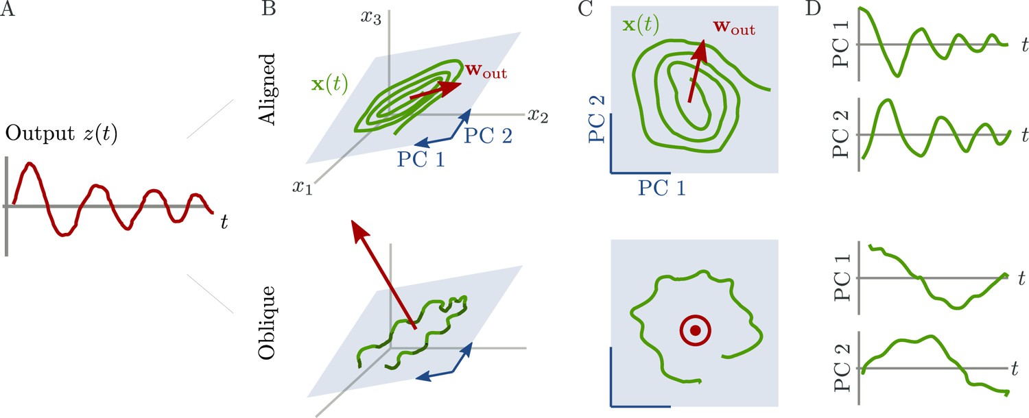
Schematic of aligned and oblique dynamics in recurrent neural networks.

(A) Output generated by both networks. (B) Neural activity of aligned (top) and oblique (bottom) dynamics, visualized in the space spanned by three neurons. Here, the activity (green) is three-dimensional, but most of the variance is concentrated along the two largest principal components (PCs) (blue). For aligned dynamics, the output weights (red) are small and lie in the subspace spanned by the largest PCs; they are hence correlated to the activity. For oblique dynamics, the output weights are large and lie outside of the subspace spanned by the largest PCs; they are hence poorly correlated to the activity. (C) Projection of activity onto the two largest PCs. For oblique dynamics, the output weights are orthogonal to the leading PCs. (D) Evolution of PC projections over time. For aligned dynamics, the projection on the PCs resembles the output $z (t)$ , and reconstructing the output from the largest two components is possible. For the oblique dynamics, such reconstruction is not possible, because the projections oscillate much more slowly than the output.

Figure 2

Download asset Open asset

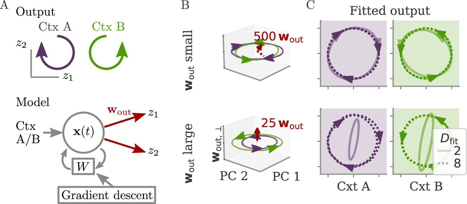
Aligned and oblique dynamics for a cycling task (Russo et al., 2018).

(A) A network with two outputs was trained to generate either clockwise or anticlockwise rotations, depending on the context (top). Our model recurrent neural network (RNN) (bottom) received a context input pulse, generated dynamics $𝐱 (t)$ via recurrent weights $W$ , and yielded the output as linear projections of the states. We trained the recurrent weights $W$ with gradient descent. (**B, C**) Resulting internal dynamics for two networks with small (top) and large (bottom) output weights, corresponding to aligned and oblique dynamics, respectively. (B) Dynamics projected on the first two principal components (PCs) and the remaining direction $𝐰_{out, ⟂}$ of the first output vector (for $z_{1}$ ). The output weights are amplified to be visible. Arrowheads indicate the direction of the dynamics. Note that for the large output weights, the dynamics in the first two PCs co-rotated, despite the counter-rotating output. (C) Output reconstructed from the largest PCs, with dimension $D = 2$ (full lines) or 8 (dotted). Two dimensions already yield a fit with $R^{2} = 0.99$ for aligned dynamics (top), but almost no output for oblique (bottom, $R^{2} = 0.005$ , no arrows shown). For the latter, a good fit with $R^{2} > 90$ % is only reached with $D = 8$ .

Figure 3

Download asset Open asset

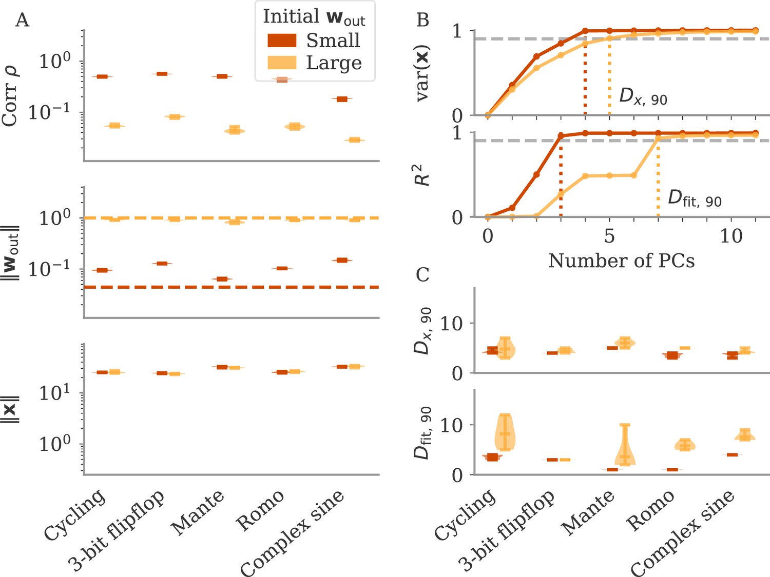
The magnitude of output weights determines regimes across multiple neuroscience tasks (Russo et al., 2018; Mante et al., 2013; Romo et al., 1999; Sussillo and Barak, 2013).

(A) Correlation and norms of output weights and neural activity. For each task, we initialized networks with small or large output weights (dark vs light orange). The initial norms $‖ 𝐰_{out} ‖$ are indicated by the dashed lines. Learning only weakly changes the norm of the output weights. Note that all y-axes are logarithmically scaled. (B) Variance of $𝐱$ explained and $R^{2}$ of reconstructed output for projections of $𝐱$ on increasing number of principal components (PCs). Results from one example network trained on the cycling task are shown for each condition. (C) Number of PCs necessary to reach 90% of the variance of $𝐱 (t)$ or of the $R^{2}$ of the output reconstruction (top/bottom; dotted lines in B). In (**A, C**) violin plots show the distribution over five sample networks, with vertical bars indicating the mean and the extreme values (where visible).

Figure 4

Download asset Open asset

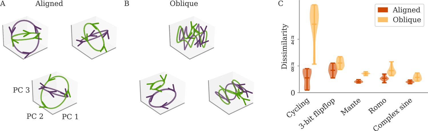
Variability between learners for the two regimes.

(**A, B**) Examples of networks trained on the cycling task with small (aligned) or large (oblique) output weights. The top left and central networks, respectively, are the same as those plotted in Figure 2. (C) Dissimilarity between solutions across different tasks. Aligned dynamics (red) were less dissimilar to each other than oblique ones (yellow). The violin plots show the distribution over all possible different pairs for five samples (mean and extrema as bars).

Figure 5

Download asset Open asset

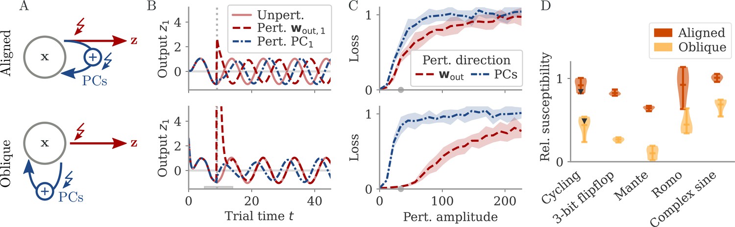
Perturbations differentially affect dynamics in the aligned and oblique regimes.

(A) Cartoon illustrating the relationship between perturbations along output weights or principal components (PCs) and the feedback loops driving autonomous dynamics. (B) Output after perturbation for aligned (top) and oblique (bottom) networks trained on the cycling task. The unperturbed network (light red line) yields a sine wave along the first output direction $z_{1}$ . At $t_{p} = 9$ , a perturbation with amplitude $‖ Δ 𝐱 ‖ = 34$ is applied along the output weights (dashed red) or the first PC (dashed-dotted blue). The perturbations only differ in the directions applied. While the immediate response for the oblique network to a perturbation along the output weights is much larger, $z_{1} (t_{p}) \approx 80$ , the long-term dynamics yield the same output as the unperturbed network. See also Appendix 1—figure 6 for more details. (C) Loss for perturbations of different amplitudes for the two networks in (B). Lines and shades are means and standard deviations over different perturbation times $t_{p} \in [5, 15]$ and random directions spanned by the output weights (red) or the two largest PCs (blue). The loss is the mean squared error between output and target for $t > 20$ . The gray dot indicates an example in (B). (D) Relative susceptibility of networks to perturbation directions for different tasks and dynamical regimes. We measured the area under the curve (AUC) of loss over perturbation amplitude for perturbations along the output weights of the two largest PCs. The relative susceptibility is the ratio between the two AUCs. The example in (C) is indicated by gray triangles.

Figure 6

Download asset Open asset

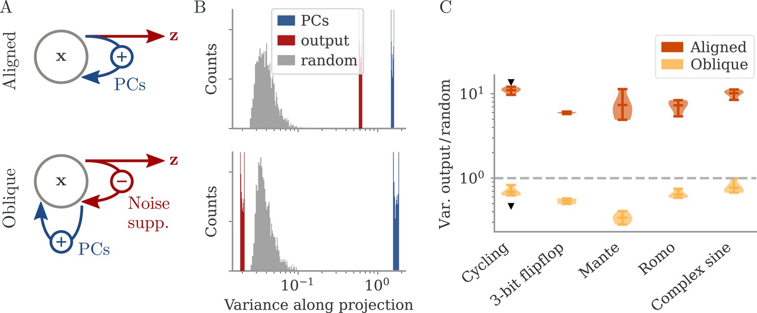
Noise suppression along the output direction in the oblique regime.

(A) A cartoon of the feedback loop structure for aligned (top) and oblique (bottom) dynamics. The latter develops a negative feedback loop which suppresses fluctuations along the output direction. (B) Comparing the distribution of variance of mean-subtracted activity along different directions for networks trained on the cycling task (see Appendix 1—figure 7): principal components (PCs) of trial-averaged activity (blue), readout (red), and random (gray) directions. For the PCs and output weights, we sampled 100 normalized combinations of either the first two PCs or the two output vectors. For the random directions, we drew 1000 random vectors in the full, $N$ -dimensional space. (C) Noise compression across tasks as measured by the ratio between variance along output and random directions. The dashed line indicates neither compression nor expansion. Black markers indicate the values for the two examples in (**B, C**). Note the log-scales in (**B, C**).

Figure 7

Download asset Open asset

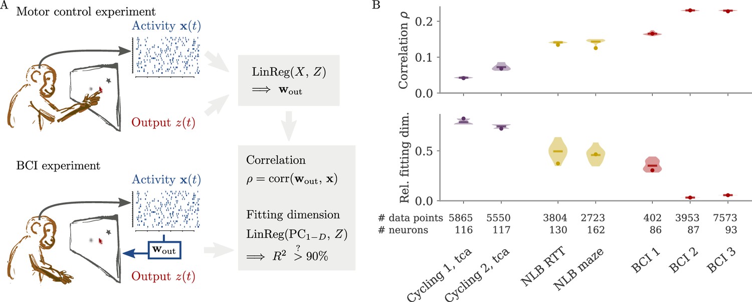
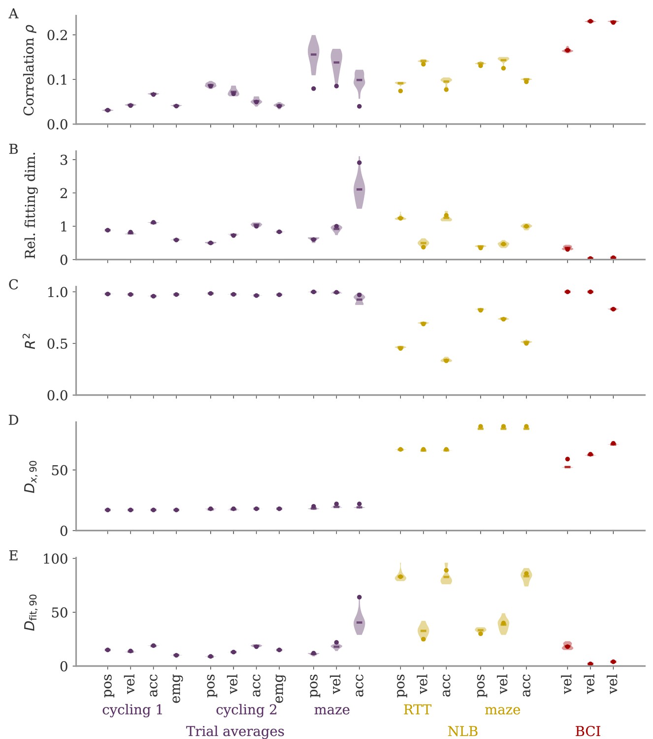
Quantifying aligned and oblique dynamics in experimental data (Russo et al., 2018; Pei et al., 2021; Golub et al., 2018; Hennig et al., 2018; Degenhart et al., 2020).

(A) Diagram of the two types of experimental data considered. Here, we always took the velocity as the output (hand, finger, or cursor). In motor control experiments (top), we first needed to obtain the output weights $𝐰_{out}$ via linear regression. We then computed the correlation $ρ$ and the reconstruction dimension $D_{fit, 90}$ , i.e., the number of principal components (PCs) of $𝐱$ necessary to obtain a coefficient of determination $R^{2} > 90$ %. In brain-computer interface (BCI) experiments (bottom), the output (cursor velocity) is generated from neural activity $𝐱 (t)$ via output weights $𝐰_{out}$ defined by the experimenter. This allowed us to directly compute correlations and fitting dimensions. (B) Correlation $ρ$ (top) and relative fitting dimension $D_{fit, 90} / D_{x, 90}$ (bottom) for several publicly available data sets. The cycling task data (purple) were trial-conditioned averages, the BCI experiments (red) and Neural Latents Benchmark (NLB) tasks (yellow) single-trial data. Results for the full data sets are shown as dots. Violin plots indicate results for 20 random subsets of 25% of the data points in each data set (bars indicate mean). See small text below x-axis for the number of time points and neurons.

Figure 8

Download asset Open asset

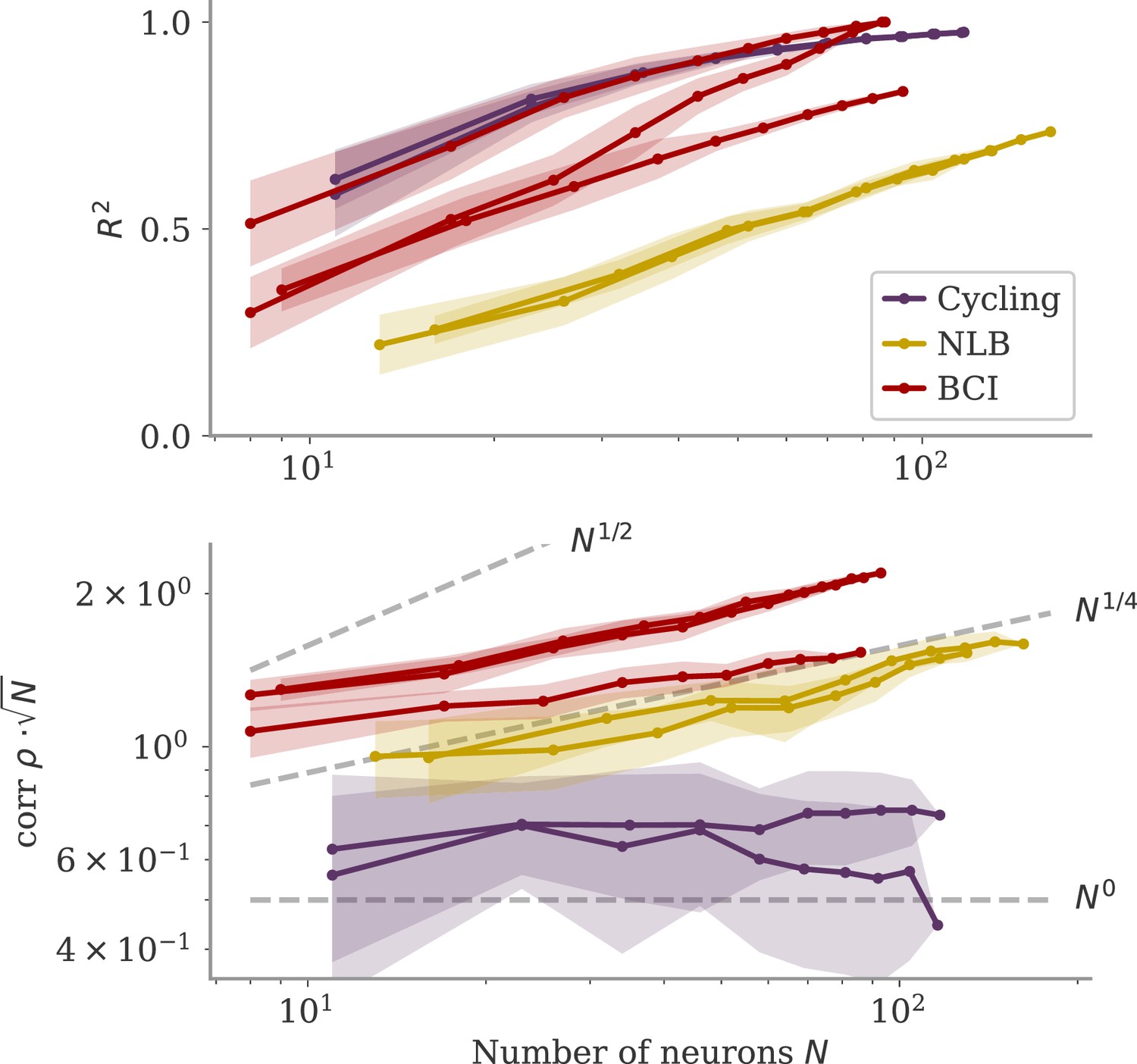
Correlation scaling with number of neurons.

Scaling of the correlation $ρ$ with the number of neurons $N$ in experimental data. We fitted the output weights to subsets of $N$ neurons and computed the quality of fit (top) and the correlation between the resulting output weight and firing rates (bottom). To compare with random vectors, the correlation is scaled by $\sqrt{N}$ . Dashed lines are $N^{p} / 2$ , for $p \in {1 / 2, 1 / 4, 0}$ for comparison. The aligned regime corresponds to $p = 1 / 2$ , and the oblique one to $p = 0$ .

Figure 9

Download asset Open asset

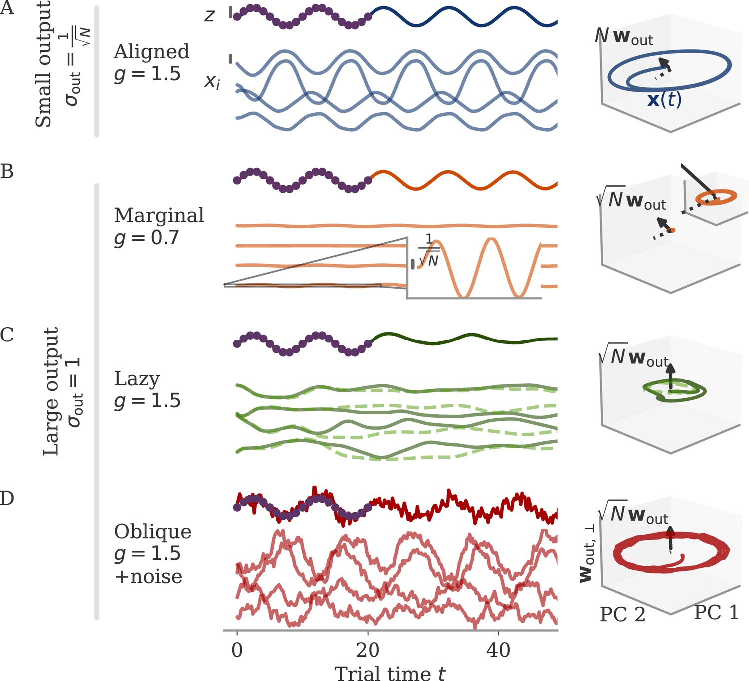
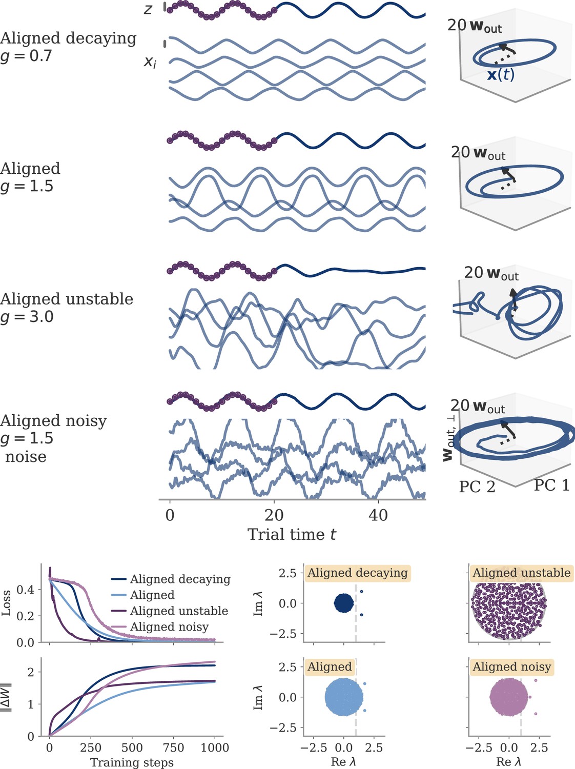
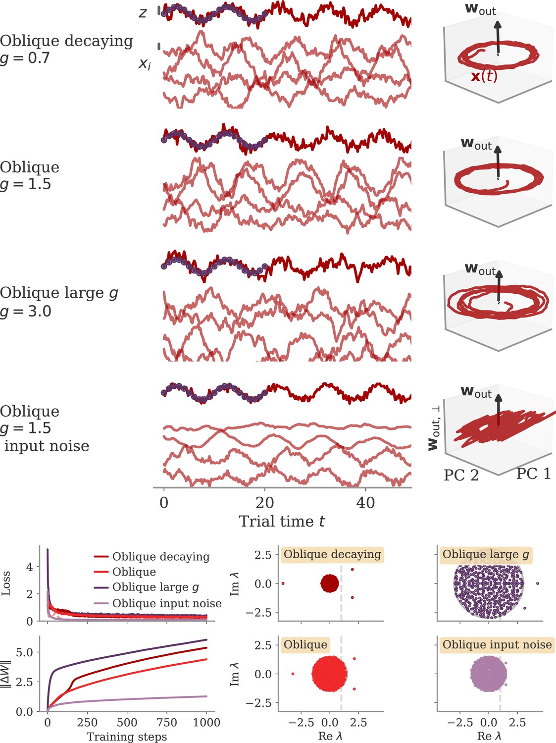
Different solutions for networks trained on a sine wave task.

All networks have $N = 512$ neurons. Four regimes: (A) aligned for small output weights, (B) marginal for large output weights, small recurrent weights, (C) lazy for both large output and recurrent weights, (D) oblique for large output weights and noise added during training. Left: Output (dark), target (purple dots), and four states (light) of the network after training. Black bars indicate the scales for output and states (length = 1; same for all regimes). The output beyond the target interval $t \in [1, 21]$ can be considered as extrapolation. The network in the oblique regime, (D), receives white noise during training, and the evaluation is shown with the same noise. Without noise, this network still produces a sine wave (not shown). Right: Projection of states on the first two principal components (PCs) and the orthogonal component $𝐰_{out, ⟂}$ of the output vector. All axes have the same scale, which allows for comparison between the dynamics. Vectors show the (amplified) output weights, dotted lines the projection on the PCs (not visible for lazy and oblique). The insets for the marginal solution (B, left and right) show the dynamics magnified by $\sqrt{N}$ .

Figure 10

Download asset Open asset

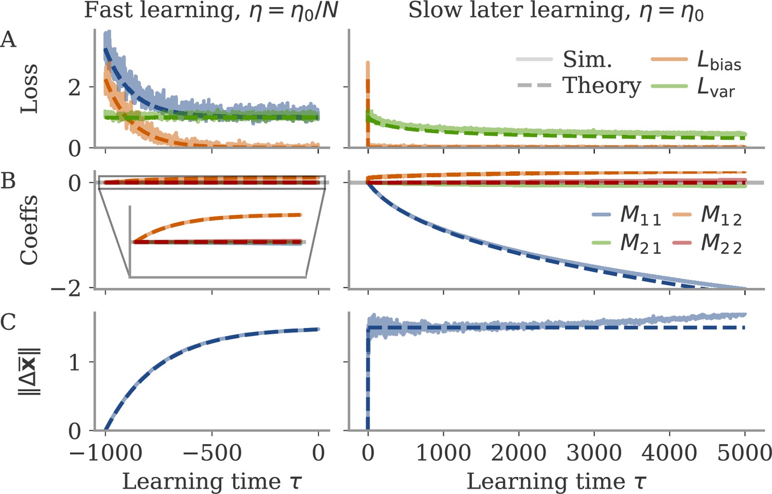
Noise-induced learning for a linear network with input-driven fixed point.

Learning separates into fast learning of the bias part of the loss (left), and slow learning reducing the variance part (right). Learning rates are $η = η_{0} / N$ and $η = η_{0}$ , respectively, with $η_{0} = 0.002$ and network size $N = 256$ . Learning epochs in the first phase are counted from –1000, so that the second phase starts at 0. In the right column, the initial learning phase with learning time steps multiplied by $1 / N$ is shown for comparison. In all plots, simulations (full lines) are compared with theory (dashed lines). (A) Loss $L = L_{bias} + L_{var}$ . The two components are obtained by averaging over a batch with 32 examples at each learning step. The full loss is not plotted in the slow phase, because it is indistinguishable from $L_{var}$ . (B) Coefficients of the 2-by-2 coupling matrix $M$ . $M_{11} = λ_{-}$ is the feedback loop along the output weights, $M_{12} = b / \sqrt{N}$ a feedforward coupling from input to output. The theory predicts $M_{21} \sim M_{22} \sim O (1 / N)$ . (C) Norm of state changes during training. The theory predicts that it remains constant during the second phase and small compared to $‖ {\overline{𝐱}}_{0} ‖ = \sqrt{N}$ . Other parameters: target $\hat{z} = 1$ , $σ_{noise} = 1$ , overlap between input and output vectors $ρ_{i o} = - 0.5 / \sqrt{N}$ .

Figure 11

Download asset Open asset

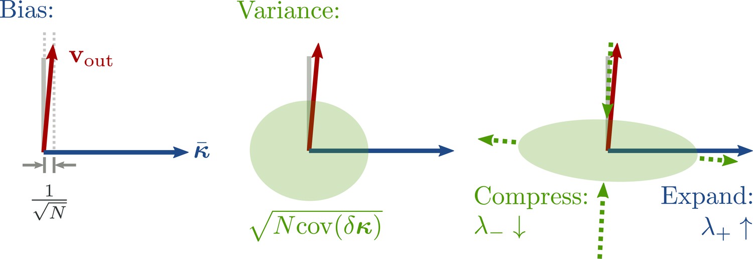
Cartoon illustrating the split into bias and variance components of the loss, and noise suppression along the output direction.

The two-dimensional subspace spanned by $U$ illustrates the main directions under consideration: the principal components (PCs) of the average trajectories (here only a fixed point $\overline{𝐱} = U \overline{𝜿}$ ), and the direction of output weights $𝐰_{out} = \frac{1}{\sqrt{N}} U 𝐯_{out}$ . Left: During learning, a fast process keeps the average output close to the target so that $L_{bias} = 0$ . Center: The variance component, $L_{var}$ , is determined by the projection of the fluctuations $δ 𝜿$ onto the output vector. Note that the noise in the low-D subspace is very small, $δ 𝜿 = O (1 \sqrt{N})$ , but the output is still affected due to the large output weights. Right: During training, the noise becomes non-isotropic. Along the average direction $\overline{𝜿}$ , the fluctuations are increased as a byproduct of the positive feedback $λ_{+}$ . Meanwhile, a slow learning process suppresses the output variance via a negative feedback $λ_{-}$ .

Figure 12

Download asset Open asset

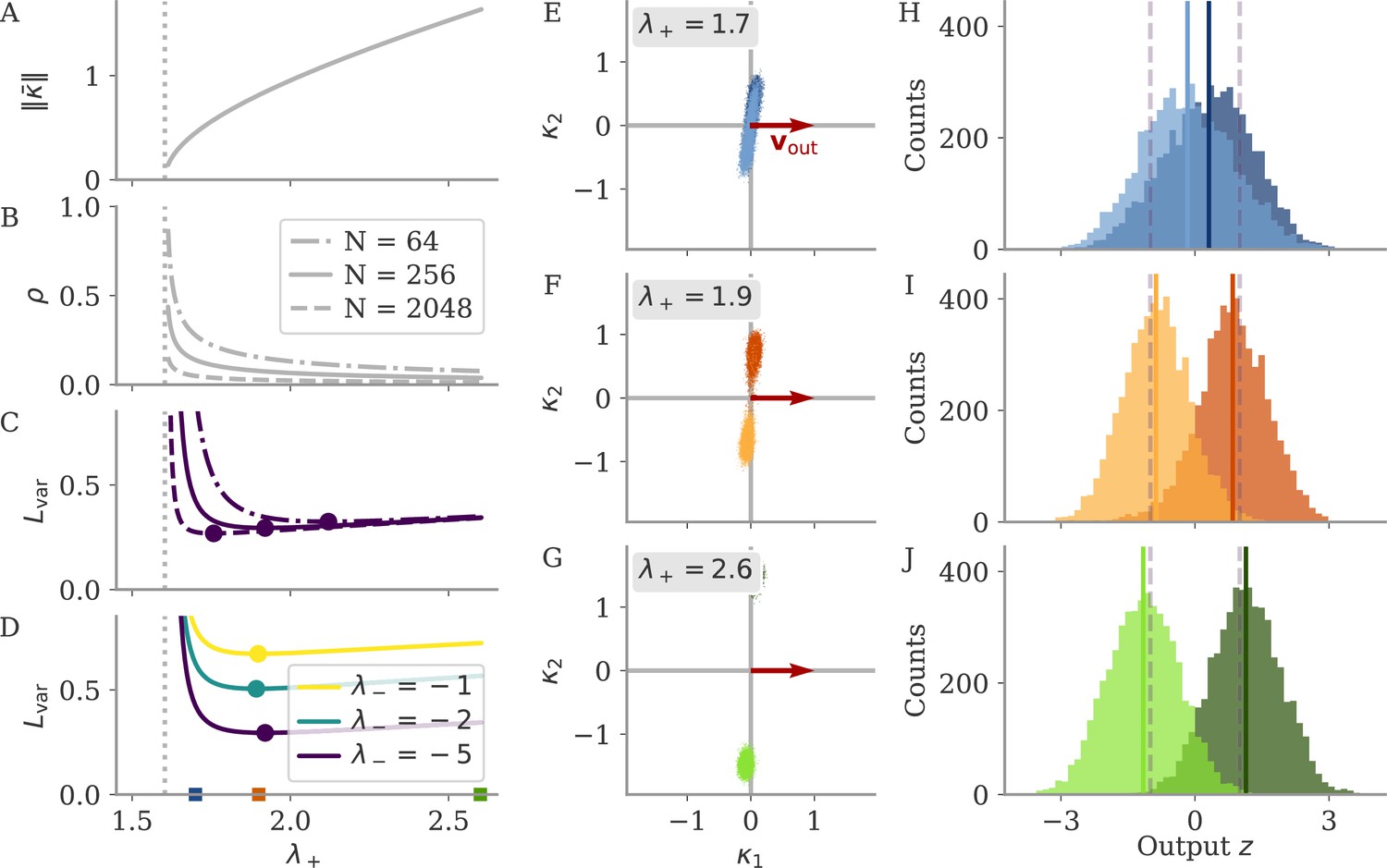
Mechanisms behind oblique solutions predicted by mean field theory.

(**A–D**) Mean field theory predictions as a function of positive feedback strength $λ_{+}$ . The dotted lines indicate $λ_{+, \min}$ , the minimal eigenvalue necessary to generate fixed points. (A) Norm of fixed point $‖ \overline{𝜿} ‖$ . (B) Correlation $ρ$ so that $L_{bias} = 0$ . (**C, D**) Loss due to fluctuations for different $λ_{-}$ or networks sizes $N$ . Dots indicate minima. (**E–G**) Latent states $𝜿$ of simulated networks for randomly drawn projections $U$ . The symmetric matrix $M$ is fixed by setting $λ_{+}$ as noted, $λ_{-} = - 5$ , and demanding $L_{bias} = 0$ (for the mean field prediction). Dots are samples from the simulation interval $t \in [20, 100]$ . (**H–J**) Histogram for the corresponding output $z$ . Mean is indicated by full lines, the dashed lines indicate the target $\hat{z}$ . Other parameters: $N = 256$ , $σ_{noise} = 1$ , $\hat{z} = 1$ .

Figure 13

Download asset Open asset

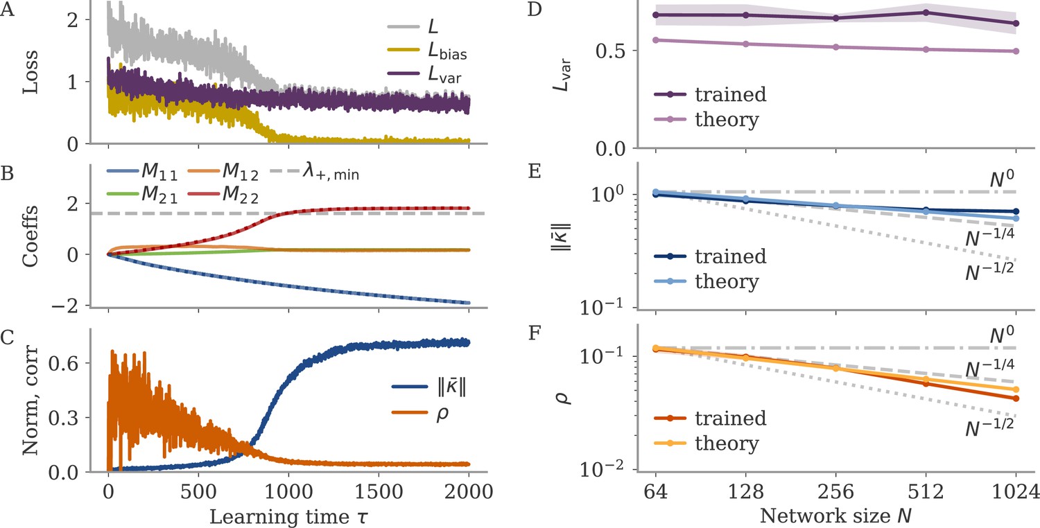
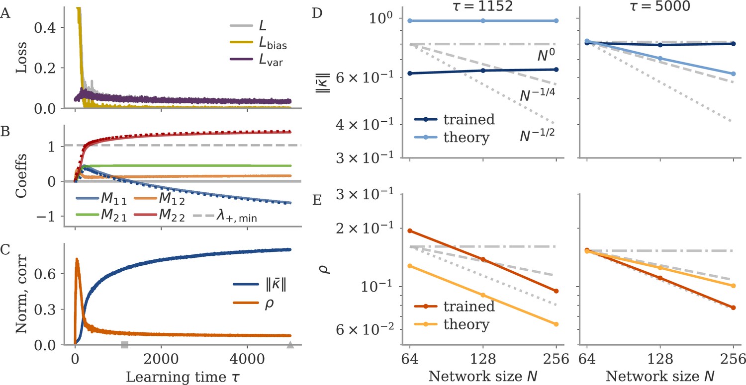
Mean field theory predicts learning with gradient descent.

(**A–C**) Learning dynamics with gradient descent for example network with $N = 1024$ neurons and with noise variance $σ_{noise}^{2} = 1$ . (A) Loss with separate bias and variance components. (B) Matrix coefficients $M_{i j}$ . The dotted lines almost identical to $M_{22}$ and $M_{11}$ indicate the eigenvalues $λ_{+}$ and $λ_{-}$ , respectively. The dashed line indicates $λ_{+, \min}$ . (C) Fixed point norm and correlation. (**D–F**) Final loss, fixed point norm, and correlation for networks of different sizes $N$ . Shown are mean (dots and lines) and standard deviation (shades) for five sample networks, and the prediction by the mean field theory. Gray lines indicate scaling as $a N^{k}$ , with $k \in {0, - 1 / 4, - 1 / 2}$ . Note the log-log axes for (**E, F**).

Figure 14

Download asset Open asset

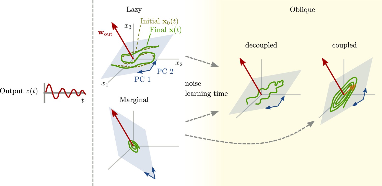
Path to oblique solutions for networks with large output weights.

Left: All networks produce the same output (Figure 1). Center: Unstable solutions that arise early in learning. For lazy solutions, initial chaotic activity is slightly adapted, without changing the dynamics qualitatively. For marginal solutions, vanishingly small initial activity is replaced with very small dynamics sufficient to generate the output. Right: With more learning time and noise added during the learning process, stable, oblique solutions arise. The neural dynamics along the largest principal components (PCs) can be either decoupled from the output (center right) or coupled (right). For decoupled dynamics, the components along the largest PCs (blue subspace) differ qualitatively from those generating the output (same as Figure 1B, bottom). The dynamics along the largest PCs inherit task-unrelated components from the initial dynamics or randomness during learning. Another possibility are oblique, but coupled dynamics (right). Such solutions don't inherit task-unrelated components of the dynamics at initialization. They are qualitatively similar to aligned solutions, and the output is generated by a small projection of the output weights onto the largest PCs (dashed orange arrow).

Appendix 1—figure 1

Download asset Open asset

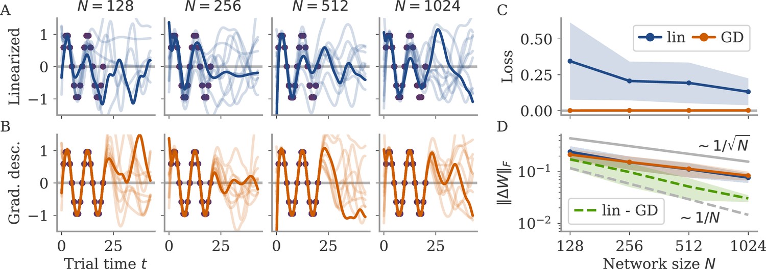
Solution to linearized network dynamics in the lazy regime.

(A) Network output for weight changes $Δ W_{lin}$ obtained from linearized dynamics for different network sizes. Each plot shows 10 different networks (one example in bold). Target points in purple. (B) Output for networks trained with gradient descent (GD) from the same initial conditions as those above. (C) Loss on the training set for the linear (lin) and GD solutions. (D) Frobenius norms of weight changes $Δ W$ of the linear and GD solutions, as well as of the difference between the two. $Δ W_{lin} - Δ W_{GD}$ (dashed green). Gray and black dashed lines for comparison of scales.

Appendix 1—figure 2

Download asset Open asset

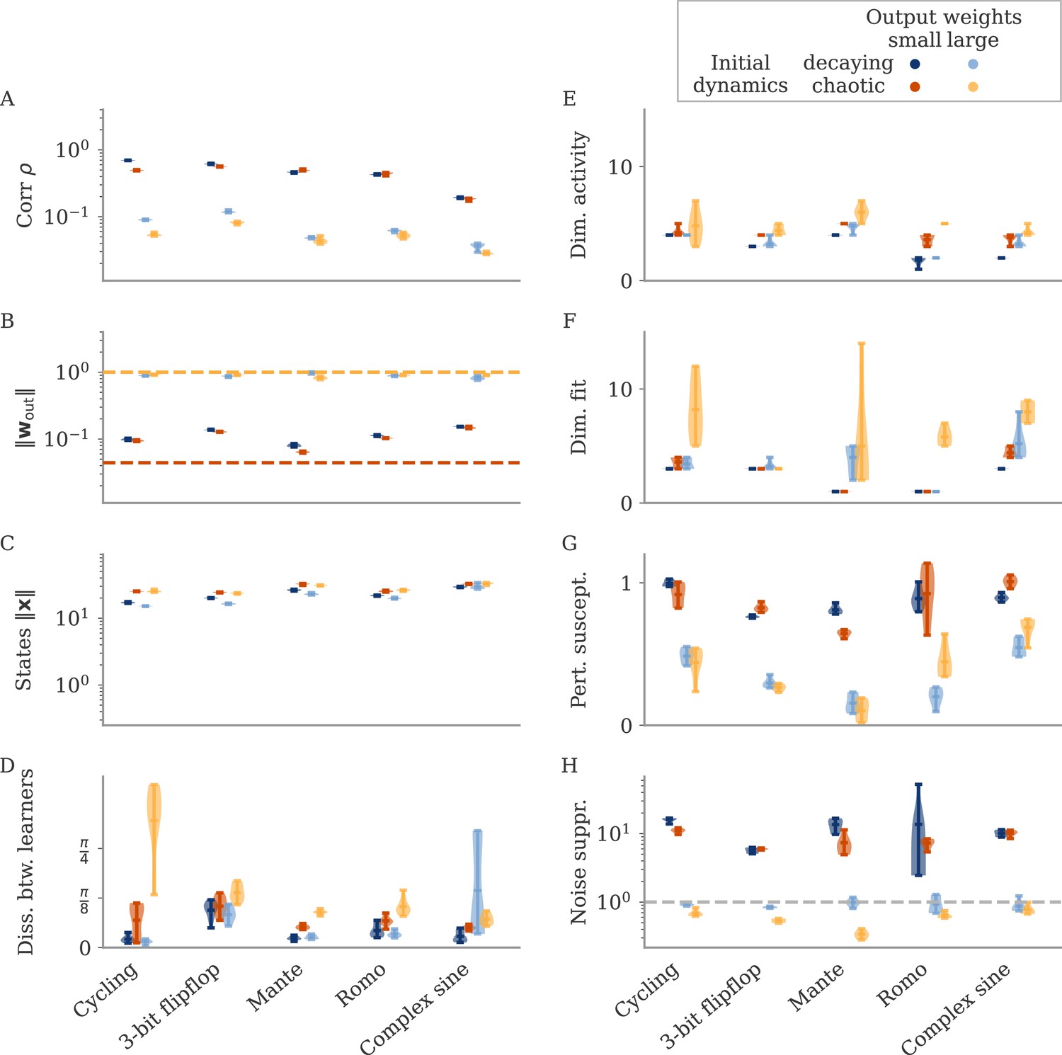
Summary of all measures for initially decaying or chaotic networks.

(A) Correlation, (B) norm of output weights, (C) norm of states, (D) dissimilarity between learners, (E) dimension of activity $D_{x, 90}$ , (F) fit dimension $D_{f i t, 90}$ , (G) susceptibility to perturbations, (H) noise suppression.

Appendix 1—figure 3

Download asset Open asset

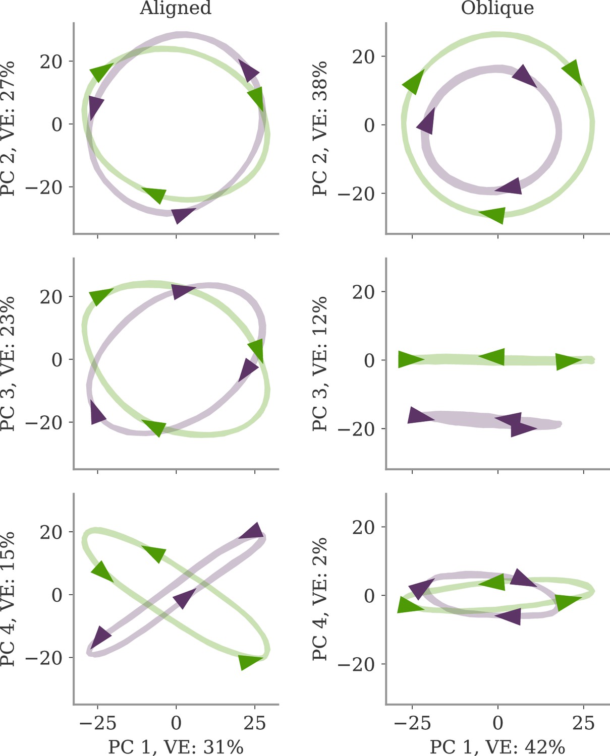
Projection of neural dynamics onto first four principal components (PCs) for the cycling task, Figure 2.

The x-axis for all plots is PC 1 of the respective dynamics (left: aligned, right: oblique). The y-axes are PCs 2–4. Axis labels indicate the relative variance explained by each PC. Arrows indicate direction. Note that there is co-rotation for the aligned network for PCs 1 and 3, as well as the counter-rotation for the oblique network for PCs 1 and 4.

Appendix 1—figure 4

Download asset Open asset

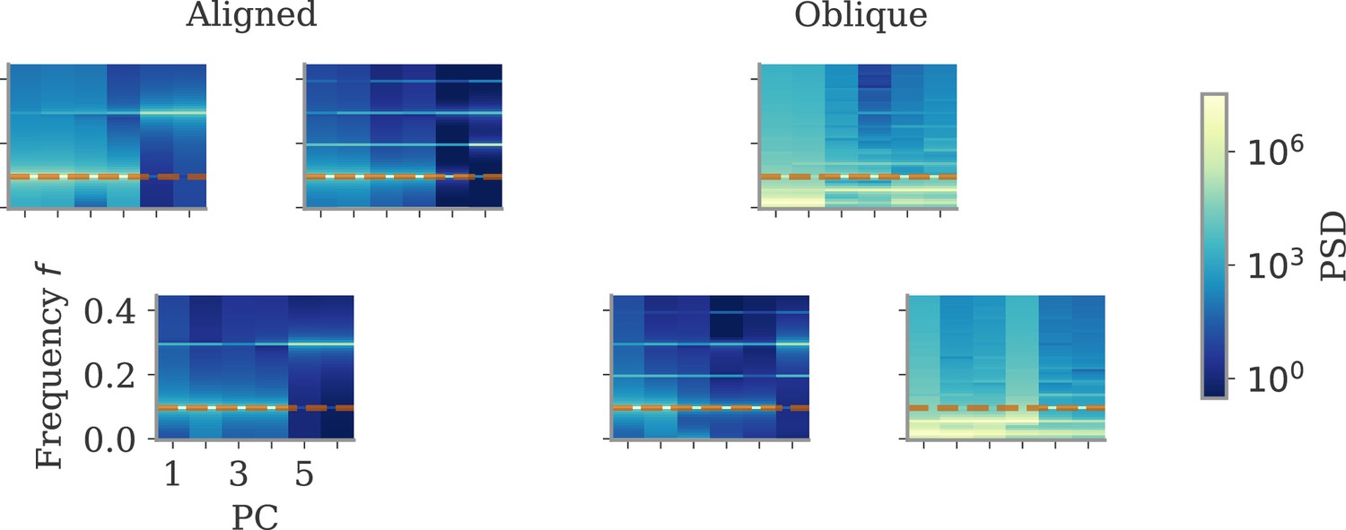
Power spectral densities for the six networks shown in Figure 4.

The dashed orange line indicates the output frequency. Note the high power for non-target frequencies in the first principal components (PCs) in some of the large output solutions.

Appendix 1—figure 5

Download asset Open asset

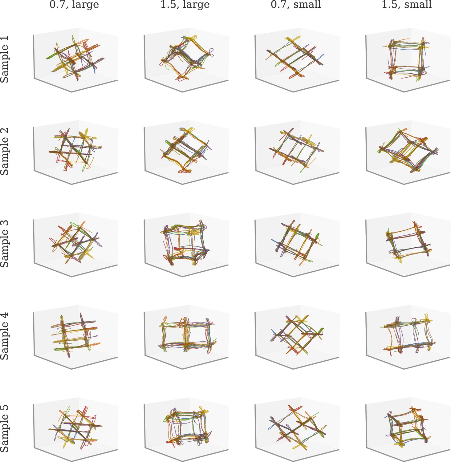
Example of task variability for the flip-flop task.

The titles in each row indicate the spectral radius $g$ of the initial recurrent connectivity ( $g > 1$ for initially chaotic, else decaying, activity), and the norm of initial output weights.

Appendix 1—figure 6

Download asset Open asset

Neural activity in response to the perturbations applied in Figure 5.

Activity is plotted in the space spanned by the leading two principal components (PCs) and the output weights $w_{o u t, 1}$ . We first show the unperturbed trajectories in each network (**A, B**), then the perturbed ones for perturbations along the first output direction (**C, D**) and along the first PC (**E, F**). The unperturbed trajectories are also plotted for comparison. Yellow dots indicate the point where the perturbation is applied. All perturbations but the one along the output for aligned lead to trajectories on the same attractor, but potentially with a phase shift. Note that in general, perturbations can also lead to the activity converging on a different attractor. Here, we see a specific example of this happening for the cycling task in the aligned regime.

Appendix 1—figure 7

Download asset Open asset

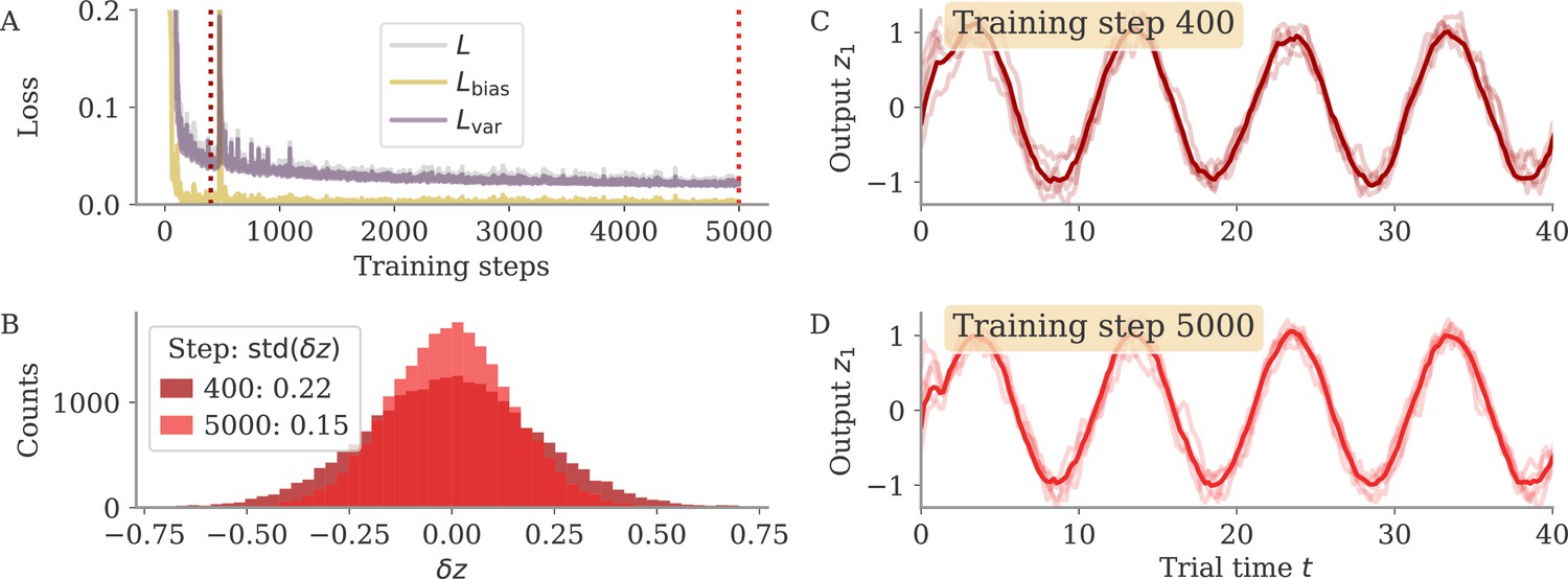
Noise compression over training time for the cycling task.

Example networks trained on the cycling tasks with $σ_{noise} = 0.2$ and $N = 256$ . The network at the end of training is analyzed in Figure 6B. (A) Full loss (gray) and decomposition in bias (golden) and variance (purple) parts over learning time. The bias part decays rapidly (the y-axis is clipped, initial loss $L_{0} = 1.4$ ), whereas the variance part needs many more training steps to decrease. Dotted lines indicate the two examples in (**B–D**). (B) Output fluctuations $δ z_{i} (t) = z_{i} (t) - {\overline{z}}_{i} (t)$ around the trial-conditioned average $\overline{z}$ . Mean is over 16 samples for each of the two trial conditions (clockwise and anticlockwise rotation). Because both output dimensions $i \in {1, 2}$ are equivalent in scale, we collected both for the histogram. (**C, D**) Example output trajectories early (C) and late (D) in learning. Shown are the mean (dark) and five samples (light).

Appendix 1—figure 8

Download asset Open asset

Fitting neural activity to different output modalities (hand position, velocity, acceleration, EMG).

Output modality is indicated by the x-ticks, the corresponding data sets by the color and the labels below. (**A, B**) Correlation and relative fitting dimension. Similar to Figure 7B, where these are shown for velocity alone. (**C–E**) Additional details. (C) Coefficient of determination $R^{2}$ of the linear regression. (D) Number of principal components (PCs) necessary to reach 90% of the variance of the neural activity $X$ . (E) Number of PCs necessary to reach 90% of the $R^{2}$ value of the full neural activity. For each output modality, the delay between activity and output is optimized. Position decodes earlier (300–200 ms) than velocity or acceleration (100–50 ms); no delay for EMG. The data $X$ is the same with each data set apart from a potential shift by the respective delay, so that dimension $D_{x, 90}$ in (D) is almost the same. Note that we also computed trial averages for the Neural Latents Benchmark (NLB) maze task to test for the effect of trial averaging. These, however, have a small sample number (189 data points, but 162 neurons), which leads to considerable discrepancy between the dots (full data) and the subsamples with only 25% of the data points, for example in the correlation (A).

Appendix 1—figure 9

Download asset Open asset

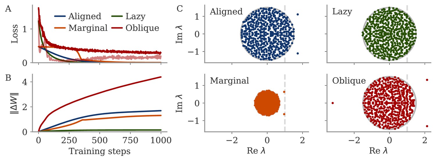
Learning curves and eigenvalue spectra for sine wave task.

(A) Loss over training steps for four networks. The light red line is the bias term of the loss for the oblique network. (B) Norm of weight changes over learning time. (C) Eigenvalue spectra of connectivity matrix $W_{f}$ after training. The dashed line indicates the stability line for the fixed point at the origin.

Appendix 1—figure 10

Download asset Open asset

The aligned regime is robust to the choice of other hyperparameters.

Appendix 1—figure 11

Download asset Open asset

The oblique regime is robust to the choice of other hyperparameters.

Appendix 1—figure 12

Download asset Open asset

Training history leads to order-one fixed point norm.

We trained recurrent neural networks (RNNs) on the example fixed point task. Similar to Figure 13, but with smaller noise $σ_{n o i s e} = 0.2$ , and with learning rate increased by 2 and number of epochs by 2.5. (**A–C**) Learning dynamics with gradient descent for one network with $N = 256$ neurons. The first 400 epochs are dominated by, $L_{b i a s}$ and $M_{11} \approx λ_{_}$ becomes *positive*. The negative feedback loop $λ_{_} < 0$ , only forms later in learning. The matrix $M$ does not become symmetric during learning. (**D, E**) Fixed point norm and correlation for different $N$ evaluated when $λ_{_} = 0$ (left) and at the end of learning (right). The time points are indicated by a square and triangle in (C), respectively. At $λ_{_} = 0$ , simulation and theory agree for the scaling: $‖ \bar{k} ‖ = O (1)$ and $ρ = O (1 / \sqrt{N})$ . At the end of training, the theory predicts a decreasing fixed point norm, but the simulated networks inherit the order-one norm from the training history.

Tables

Table 1

Task, simulation, and network parameters for Figures 3—6.

Parameter	Symbol	Cycling	Flip-flop	Mante	Romo	Complex sine
# inputs	$N_{i n}$	2	3	4	1	1
# outputs	$N_{o u t}$	2	3	1	1	1
Trial duration	$T$	72	25	48	29	50
Fixation duration	$t_{fix}$	0	$U (0, 1)$	3	$U (1.3)$	0
Stimulus duration	$t_{stim}$	1	1	20	1	50
Stimulus delay	$t_{sd}$	–	$U (3, 10)$	–	$U (2, 12)$	–
Decision delay	$t_{delay}$	1	2	5	4	0
Decision duration	$t_{dec}$	71	$t_{sd}$	20	8	50
Simulation time step	$Δ t$	– 0.2 –
Target time step	$Δ t_{target}$	1.0	1.0	1.0	1.0	0.2
Activation noise	$\sqrt{2} σ_{noise}$	0.2	0.2	0.05	0.2	0.2
Initial state noise	$σ_{init}$	– 1.0 –
Network size	$N$	– 512 –
# training epochs		1000	4000	4000	6000	6000
Learning rate aligned	$η_{0}$	0.02	0.005	0.002	0.005	0.005
Learning rate oblique	$η_{0}$	0.02	0.01	0.02	0.01	0.005
Batch size		– 32 –