Mesoscale functional organization and connectivity of color, disparity, and naturalistic texture in human second visual area
- Department of Psychological and Cognitive Sciences, Tsinghua University, China
- State Key Laboratory of Brain and Cognitive Science, Institute of Biophysics, Chinese Academy of Sciences, China
- University of Chinese Academy of Sciences, China
- Department of Psychology and Cognition and Human Behavior Key Laboratory of Hunan Province, Hunan Normal University, China
- Center for Mind & Brain Sciences, Hunan Normal University, China
- THU-IDG/McGovern Institute for Brain Research, Tsinghua University, China
- Institute of Artificial Intelligence, Hefei Comprehensive National Science Center, China
Figures
Figure 1 with 1 supplement
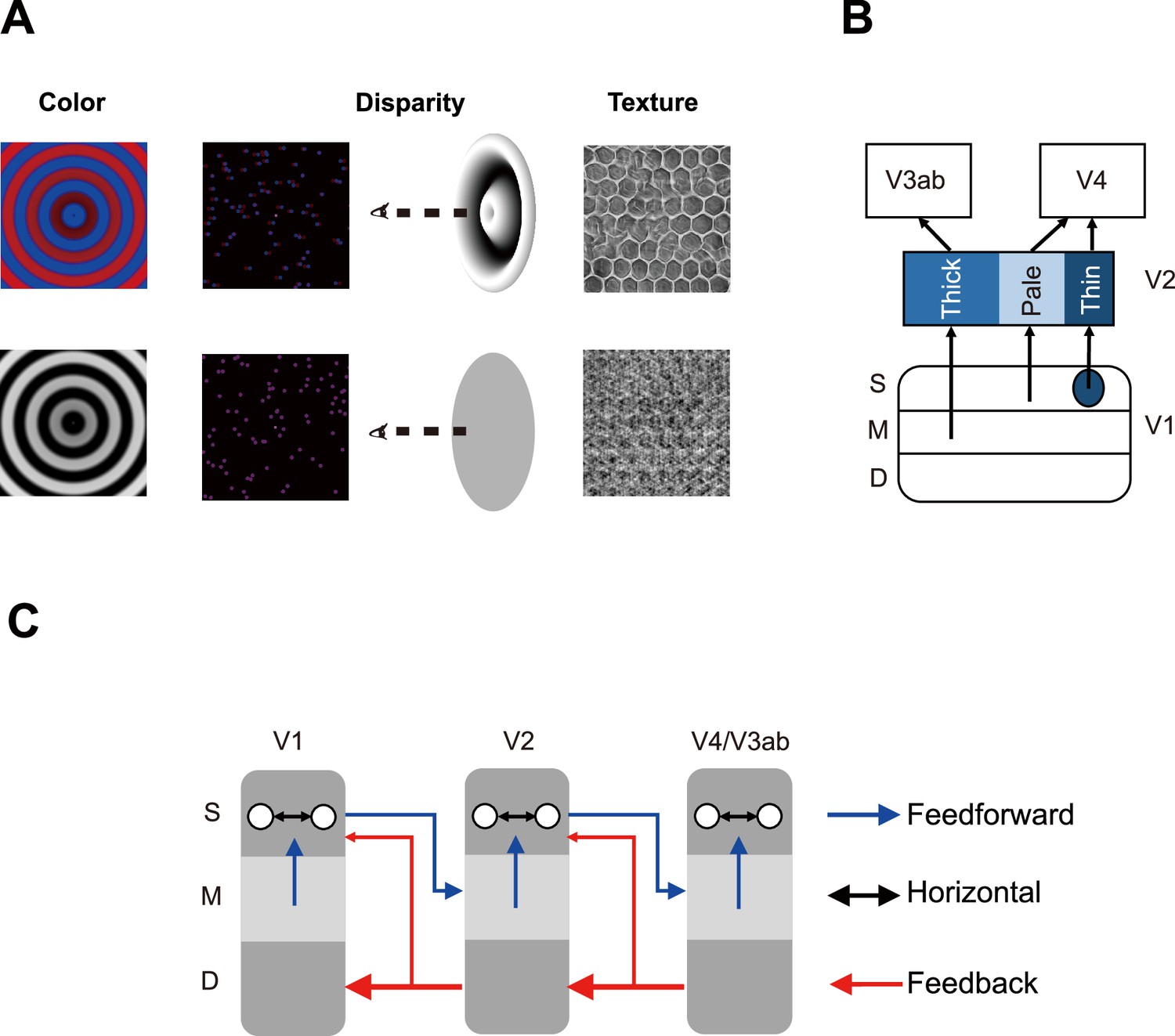
Visual stimuli and model of layer-specific neural circuitry.
(A) Visual stimuli for the fMRI experiments. Left: chromatic and achromatic gratings for the color experiment; Middle: disparity-defined grating and zero-disparity disc from random dots for the disparity experiment; Right: naturalistic texture and spectrally matched noise for the texture experiment. (B) Parallel information processing pathways in the early visual areas. (C) Layer-specific neural circuitry of feedforward, feedback, and horizontal connections in the early visual areas. S: superficial layers; M: middle layers. D: deep layers.
Figure 1—figure supplement 1
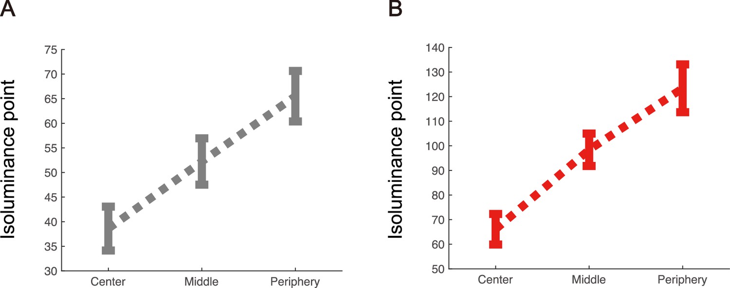
Results of isoluminance adjustment.
RGB indices of gray (A) and red (B) that match the luminance of maximum blue values across three eccentricities. Error bars indicate 1 SEM across ten subjects.
Figure 2 with 9 supplements
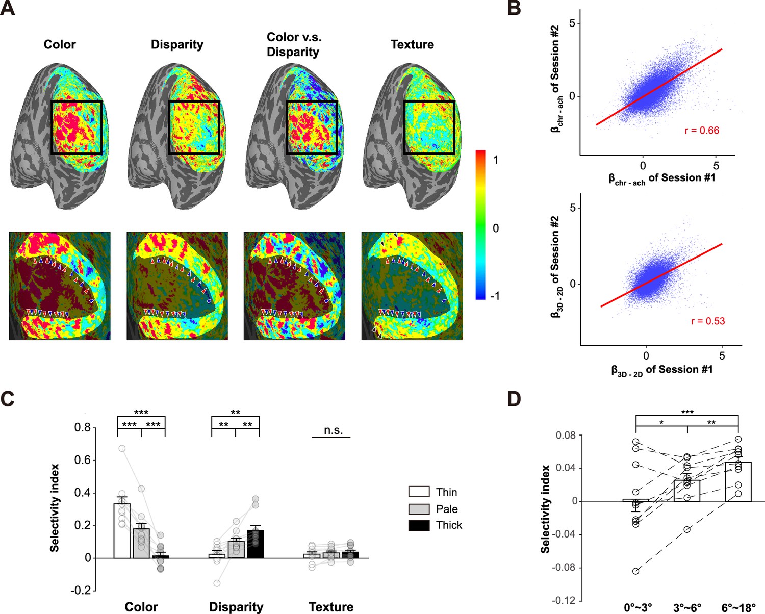
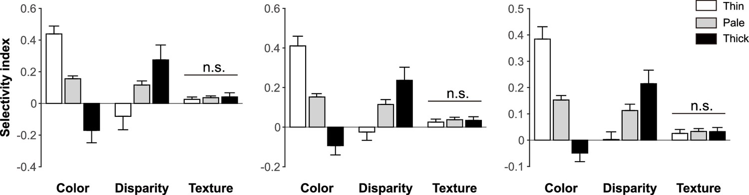
Response selectivity of color, disparity, and naturalistic texture in V2.
(A) Activation maps in a representative subject (S09). The scale bar denotes percent signal change of BOLD response. From left to right: Chr – Ach (color), 3D – 2D (disparity), color – disparity, T – N (texture). The bottom panels show enlarged activations in the black square. The highlighted region in the bottom panels represents area V2. Color-selective and disparity-selective stripe-shaped activations arranged perpendicular to the V1-V2 border. Red arrowheads denote the location of color-selective (thin) stripes and blue arrowheads denote the location of disparity-selective (thick) stripes. Black arrowheads in the fourth column highlight the texture-selective activations in anterior V2 (corresponding to peripheral visual field). The regions of interest (ROIs) for pale stripes were defined as vertices in-between adjacent thin and thick stripes (see ‘Materials and methods’ for details). (B) Inter-session correlations for the color- and disparity-selective functional maps in S09. Each blue dot represents one vertex on V2 surface. (C) Selectivity indices for color, disparity and naturalistic texture in different types of columns. Error bar indicates 1 SEM across subjects. **p<0.01, ***p<0.001. n.s.: none significance. Circles represent data from individual participants. (D) Texture selectivity at different eccentricities. Error bars represent 1 SEM across ten participants. *p<0.05, **p<0.01, ***p<0.001.
Figure 2—figure supplement 1
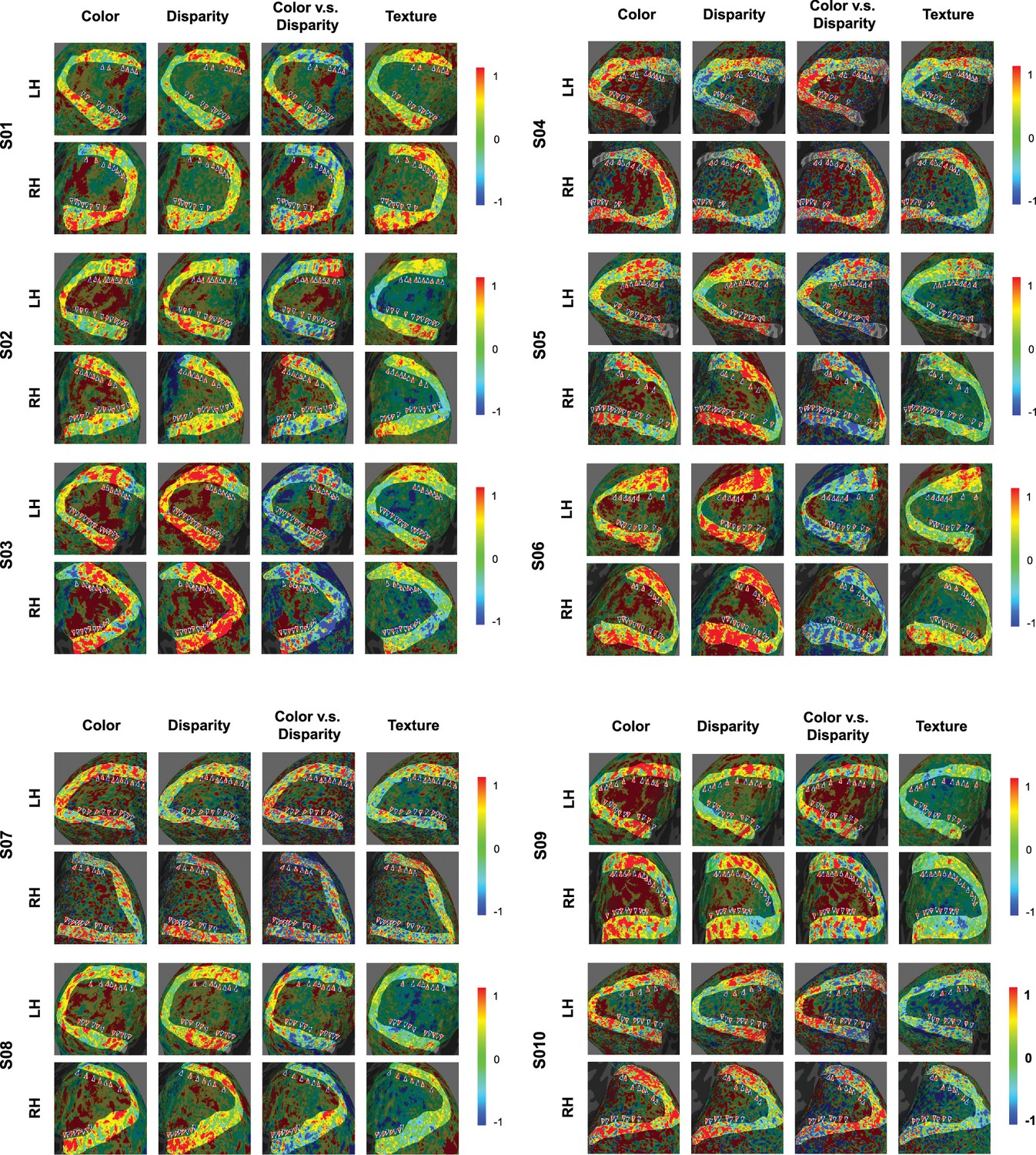
The functional maps in V2 for all 10 subjects.
The scale bar denotes percent signal change of BOLD response. Color-selective thin and disparity-selective thick stripes were denoted by red and blue arrows, respectively. The number of stripes in each category is summarized in Figure 2—figure supplement 1—source data 1. LH: left hemisphere; RH: right hemisphere.
-
Figure 2—figure supplement 1—source data 1
The number of stripes in manually defined ROIs.
- https://cdn.elifesciences.org/articles/93171/elife-93171-fig2-figsupp1-data1-v1.docx
Figure 2—figure supplement 2
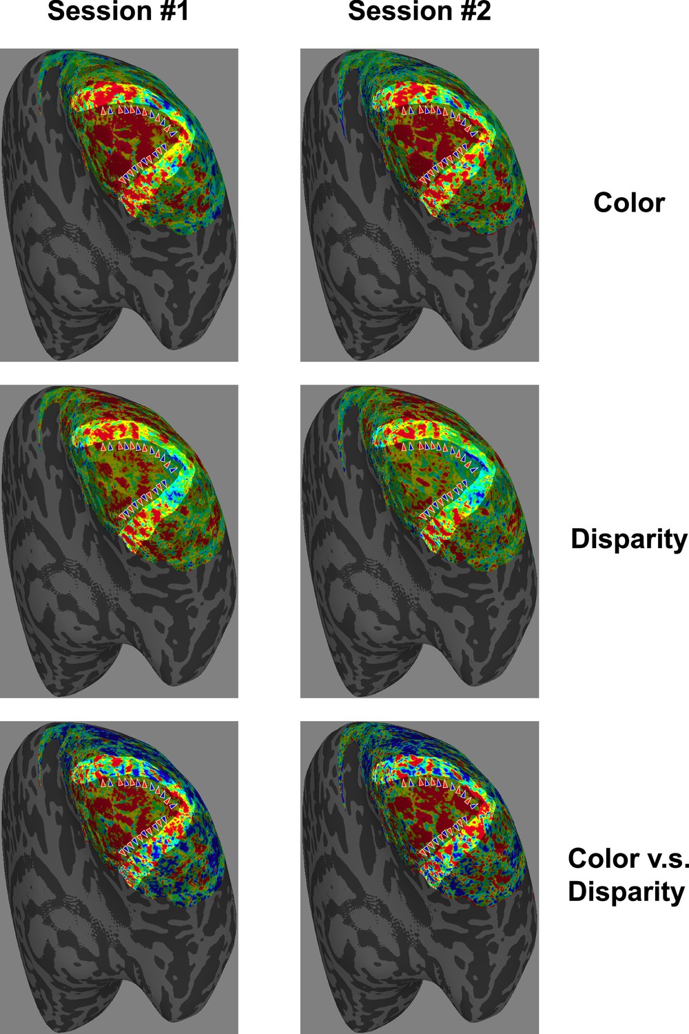
Test-retest activation patterns for color and disparity experiments in a subject (S09).
Color-selective thin and disparity-selective thick stripes are denoted by red and blue arrows, respectively.
Figure 2—figure supplement 3
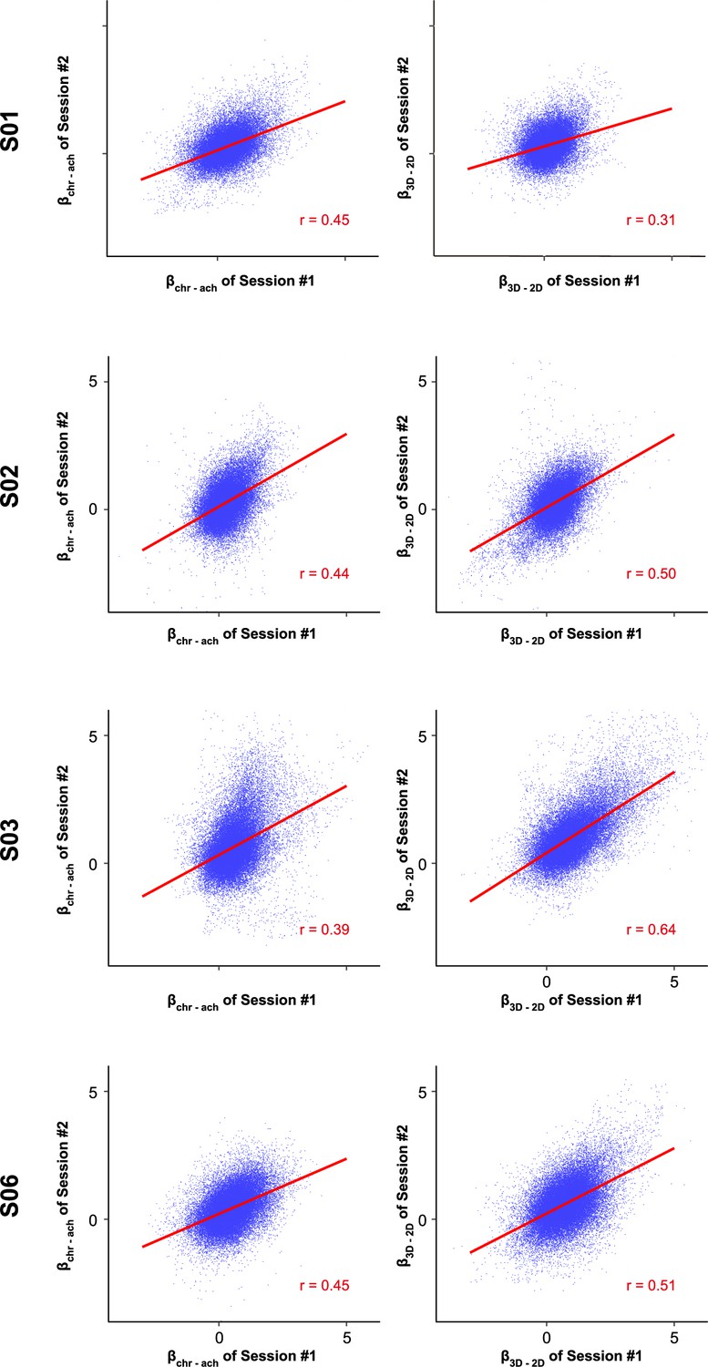
Inter-session correlations for the color- and disparity-selective activation maps in four subjects who scanned both color and disparity experiments in 2 days.
The results for S09 are shown in Figure 2.
Figure 2—figure supplement 4
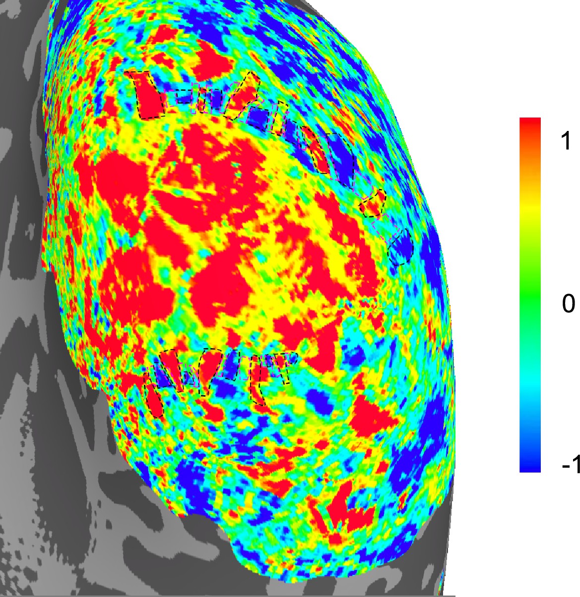
The manually defined ROIs for disparity-selective thick, color-selective thin stripes, and the pale stripes in-between in a representative subject (S09).
The scale bar denotes percent signal change of BOLD response. The stripes are framed with dashed lines. Black: thin and thick stripes (Figure 2A); purple: pale stripes.
Figure 2—figure supplement 5
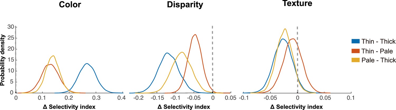
The bootstrapped distributions of stimulus-selectivity indices in different types of column ROIs.
Dashed lines indicate zero selectivity. Color- and disparity-selective indices both show significant differences across three stripes. Texture-selective index shows non-significant difference across different stripes.
Figure 2—figure supplement 6
Feature selectivity in CO-stripes under different ROI-definition thresholds.
From left to right: 10%, 20%, and 30% of extreme voxels. We defined the stripe ROIs using different thresholds to investigate whether the results were independent of the threshold for ROI definition. Specifically, we ranked the voxels in manually defined stripe ROIs by the color-disparity response. We then defined the lowest 10% as the thick stripe voxels, the highest 10% as thin stripe voxels, and the middle 10% as pale stripe voxels. Additionally, we adjusted the thresholds to select 20% or 30% of extreme voxels to define the three stripes (with 30% being the least strict threshold). Notably, in all threshold conditions, there was no significant difference in texture selectivity across different stripes. Error bars indicate 1 SEM across ten subjects.
Figure 2—figure supplement 7
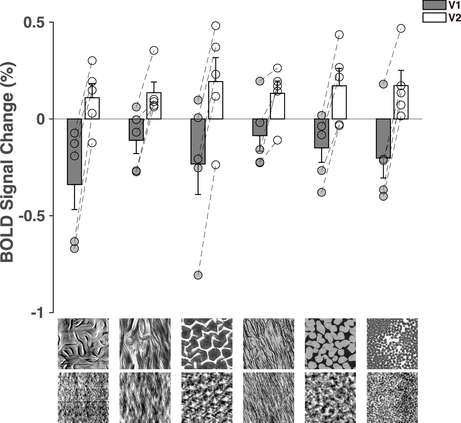
The response difference between texture and noise in the 3T fMRI experiment.
The six naturalistic textures were used as stimuli in both 3T and 7T fMRI experiments. MRI data were collected using a 3T Siemens scanner (Prisma) with a 32-channel phased-array coil. Stimuli were back- projected via an MRI-safe projector (spatial resolution: 1024 × 768, refresh rate: 60 Hz). Anatomical volumes were acquired with a T1-weighted MPRAGE sequence at 1 mm isotropic resolution. Functional data were collected with a gradient echo planar imaging sequence (TE = 34 ms; TR = 2 s; FOV = 200 × 200 mm2; matrix = 100 × 100; flip angle = 90°; slice thickness = 2 mm; 72 axial slices). Each run consisted of thirty 24 s stimulus blocks, starting and ending with 16 s fixation periods. Blocks of naturalistic texture and spectrally matched noise stimuli were presented alternatively. In each block, a random sequence of images from one texture family (naturalistic texture or spectrally matched noise) were presented at 5 Hz. There were 15 pairs of naturalistic texture and spectrally matched noise in one run. Eight runs were collected for two subjects while four runs for the other three subjects. MRI data analyses were similar as those in the 7T experiment. Error bars indicate 1 SEM across ten subjects.
Figure 2—figure supplement 8
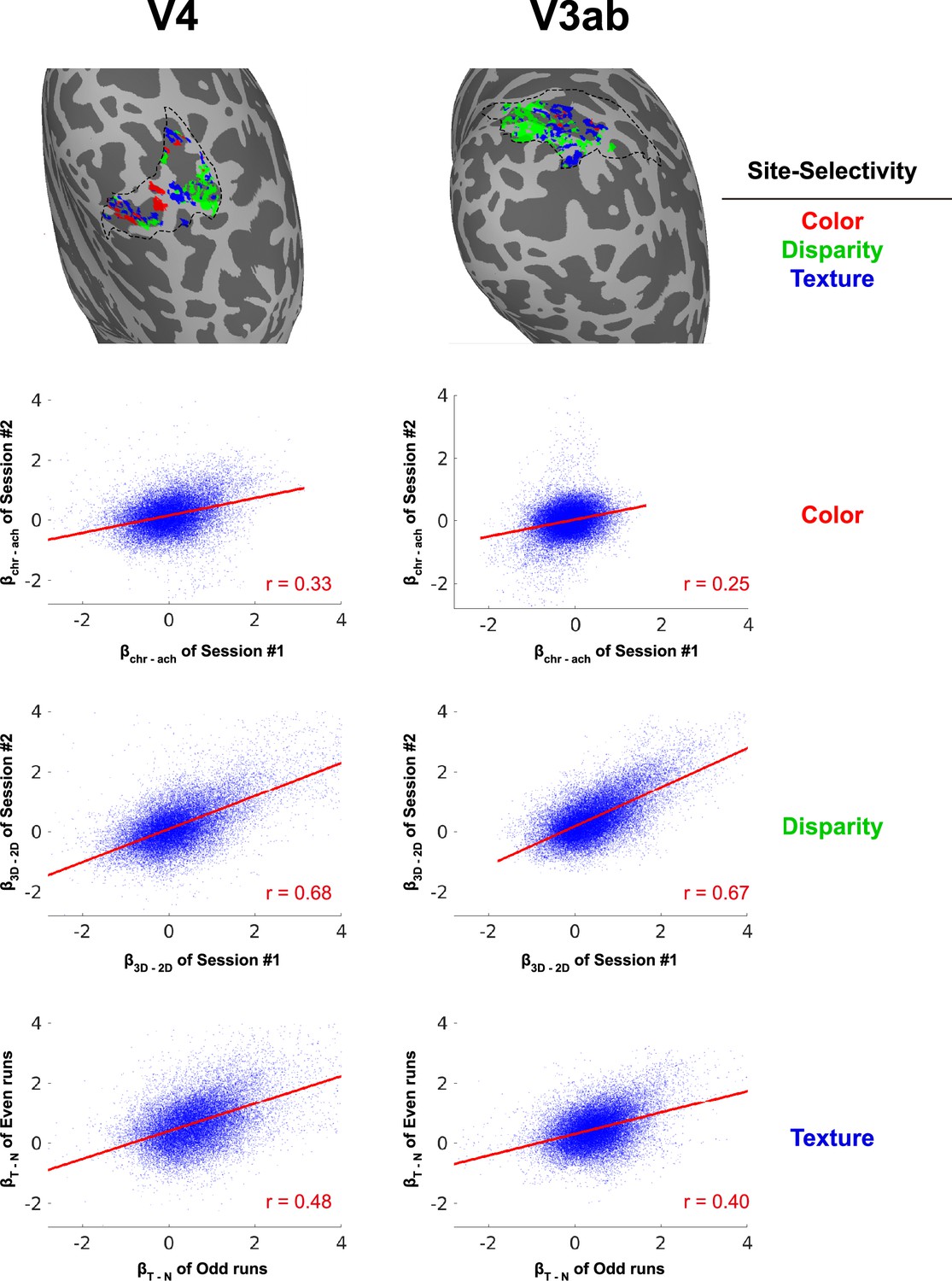
Maps showing selectivity for color, disparity and naturalistic texture in V4 and V3ab in a subject (S01).
Selectivity maps for three experiments were initially thresholded at p<0.05 and then normalized by linearly scaling the values from 0 to 1. A vertex was classified as selective for a particular feature (i.e., either color, disparity or texture) if its normalized value was times greater than the value for any other feature. Inter-session correlations were also calculated for the activation maps showing selectivity for color-selective, disparity-selective, and texture-selective in V4 (left panel) and V3ab (right panel).
Figure 2—figure supplement 9
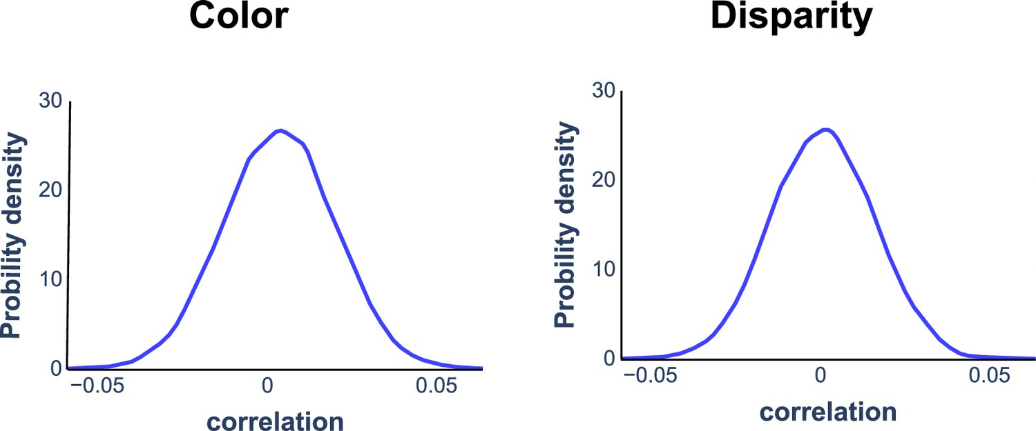
Null distributions of pattern correlation coefficients from Monte Carlo simulation.
Figure 3 with 2 supplements
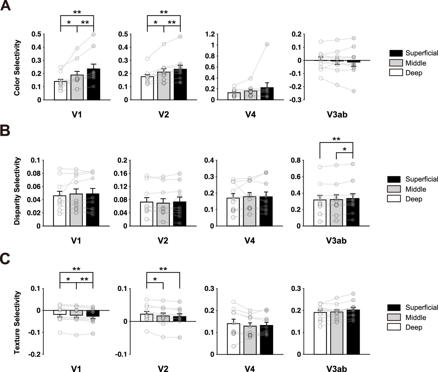
Layer-specific response selectivity for color (A), disparity (B), and naturalistic texture (C).
Error bars indicate 1 SEM across ten subjects. *p<0.05, **p<0.01. See Figure 3—figure supplement 1 for the original BOLD response across cortical depth.
Figure 3—figure supplement 1
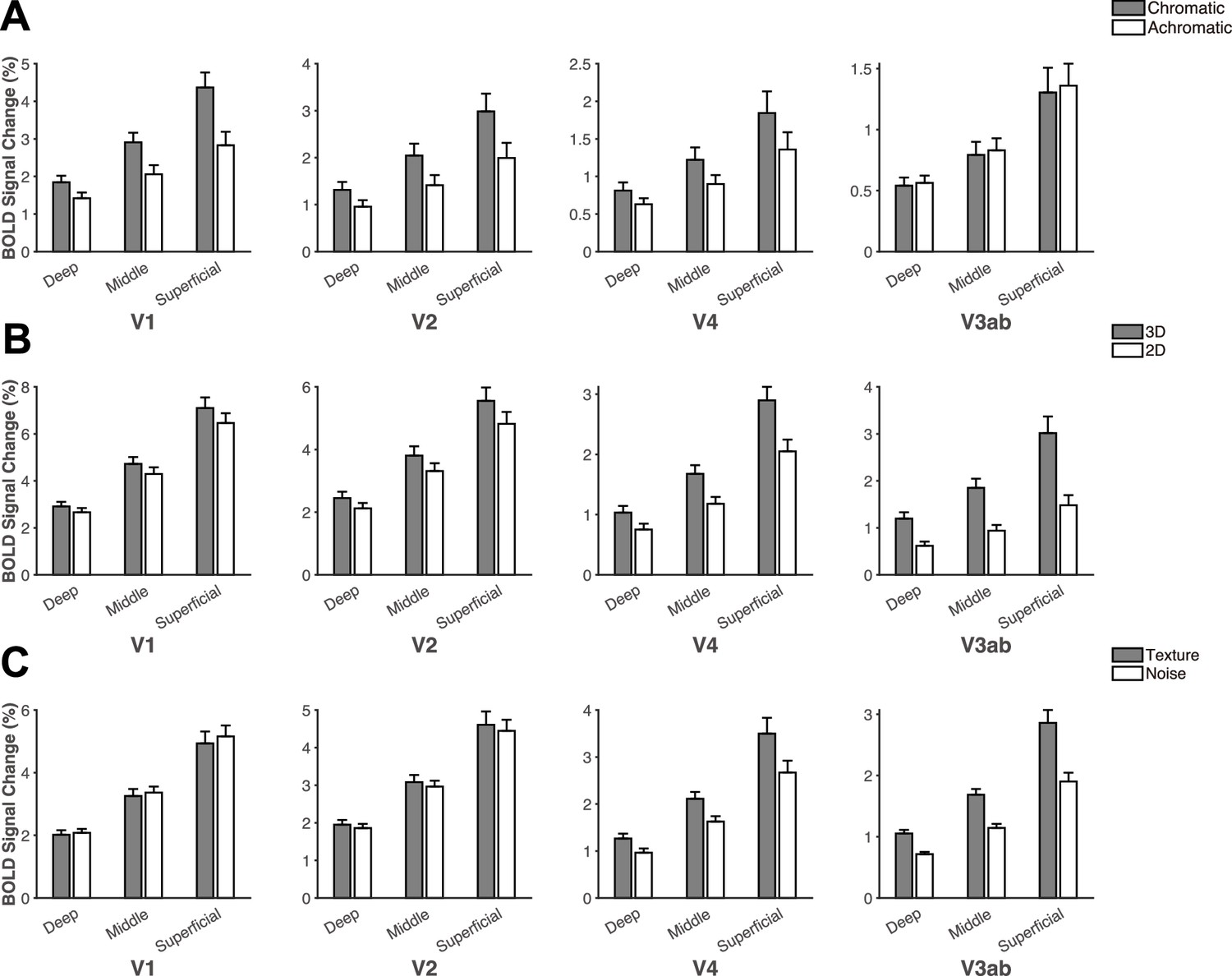
Raw BOLD signal changes for calculating layer-specific selectivity indices in color (A), disparity (B), and texture experiment (C).
Error bars indicate 1 SEM across ten subjects.
Figure 3—figure supplement 2
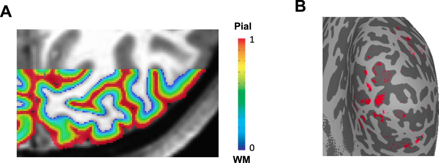
Illustrations of depth map (A) and pial vein removal (B).
Red pixels in (B) represent vertices with extremely large signal changes (top 5%) that were excluded.
Figure 4
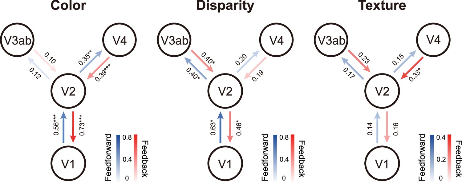
Layer-specific feedforward and feedback informational connectivity of color, disparity, and naturalistic texture.
Numbers denote the mean values of connection (Pearson’s r) across all subjects. *p<0.05, **p<0.01, ***p<0.001 after false discovery rate correction.
Author response image 1

Retinotopic ROIs defined by the Benson atlas (left) and the polar angle map (right) of the representative subject.
Black lines denote the boundaries of early visual areas based on the retinotopic map from the subject.
Author response image 2
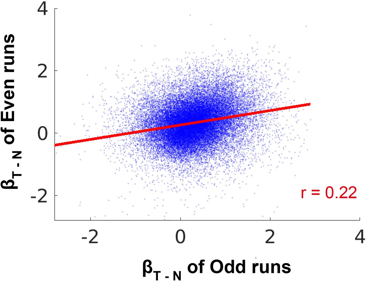
Split-half correlations for the texture-selective activation maps in a representative subject (S01) in V2.
Author response image 3

Split-half analysis of informational connectivity.
Tables
Key resources table
| Reagent type (species) or resource | Designation | Source or reference | Identifiers | Additional information |
|---|---|---|---|---|
| Software, algorithm | FreeSurfer (version 6.0) | https://surfer.nmr.mgh.harvard.edu | RRID:SCR_001847 | |
| Software, algorithm | AFNI | http://afni.nimh.nih.gov/afni/ | RRID:SCR_005927 | |
| Software, algorithm | ANTs | Avants et al., 2011 | RRID:SCR_004757 | |
| Software, algorithm | mripy | https://pypi.org/project/mripy/; herrlich10, 2025 | ||
| Software, algorithm | MATLAB | MathWorks | RRID:SCR_001622 | |
| Software, algorithm | Psychophysics toolbox | http://psychtoolbox.org/ | RRID:SCR_002881 | |
| Software, algorithm | JASP | https://jasp-stats.org/ | RRID:SCR_015823 | |
| Software, algorithm | Portilla-Simoncelli model | Portilla and Simoncelli, 2000 | - | Used for synthesizing naturalistic texture |
| Other | 7T MAGNETOM MRI scanner | Siemens Healthineers | - | MRI data collection |
| Other | 32-channel receive, 4-channel transmit open-face surface coil | Sengupta et al., 2016 | - | Custom-built open-face visual coil |
| Other | Custom anaglyph spectacles (red and cyan) | This paper | - | Used for disparity experiment |
Additional files
Download links
A two-part list of links to download the article, or parts of the article, in various formats.
Downloads (link to download the article as PDF)
Open citations (links to open the citations from this article in various online reference manager services)
Cite this article (links to download the citations from this article in formats compatible with various reference manager tools)
Mesoscale functional organization and connectivity of color, disparity, and naturalistic texture in human second visual area
eLife 13:RP93171.
https://doi.org/10.7554/eLife.93171.3


