On the pH-dependence of α-synuclein amyloid polymorphism and the role of secondary nucleation in seed-based amyloid propagation
- Institute of Molecular Physical Science, Switzerland
- Scientific Center for Optical and Electron Microscopy, Switzerland
- Robert P. Apkarian Integrated Electron Microscopy Core, Emory University, United States
- Institute of Molecular Systems Biology, ETH Zürich, Switzerland
Figures
Figure 1
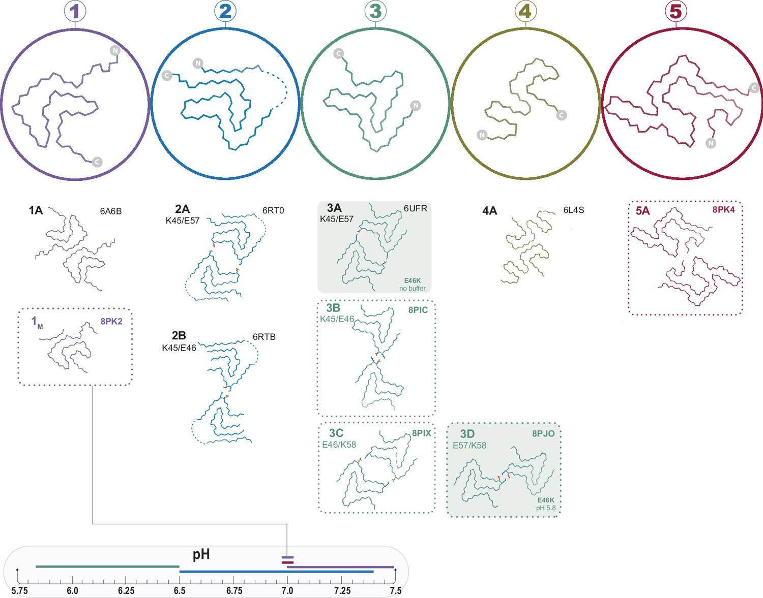
The polymorphs formed in vitro by wild-type α-synuclein (α-Syn).
The numbered backbone Cα traces depicting a single chain from each of the five types of polymorphs that have been reported to form in vitro with wild-type α-Syn but without cofactors. The interface variants of each type are also shown by a representative structure from the PDB or from one of the structures reported in this manuscript (boxed in dotted lines). Two mutant structures for the Type 3 fold are included in order to show the special 3A and 3D interfaces that form for these mutants (shaded background). The observed pH-dependence of each of the polymorphs described in this manuscript is indicated by the colored line above the pH scale (or, in the case of the 1M polymorph reported here, by a line connecting it to the scale).
Figure 2
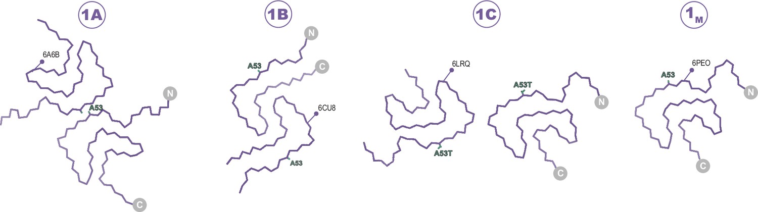
The Type 1 polymorphs.
Backbone Cα traces showing the four different interface polymorphs of Type 1, including 1B whose fold is not classically Type 1 but whose name is kept for consistency with previous publications. The 1C polymorph is only formed by mutants at the 1A interface (here A53T) and so residue 53 is highlighted in each structure.
Figure 3
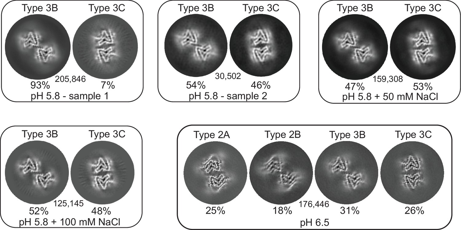
3D classification of particles in fibril samples from various conditions.
The 3D classes obtained in RELION for five different fibril samples grown at pH 5.8 and 6.5 in PBS with or without additional NaCl are shown. Each box presents the output classes from one sample with the ratio of the polymorphs determined by the number of particles assigned to each class and the total number of particles used indicated in the center of the box. Classifications were performed with input models for each of the output classes plus one additional cylindrical model (not shown) to provide a ‘junk’ class for particles that do not fit any of the main classes. The particles that went into the ‘junk’ class were not included in determining that ratios of particles in the main classes. In the case of the pH 6.5 data, the fibril classes were better separated by filament subset selection in RELION (see Methods and Table 1) and the four classes shown represent the output from individual 3D refinements.
Figure 4
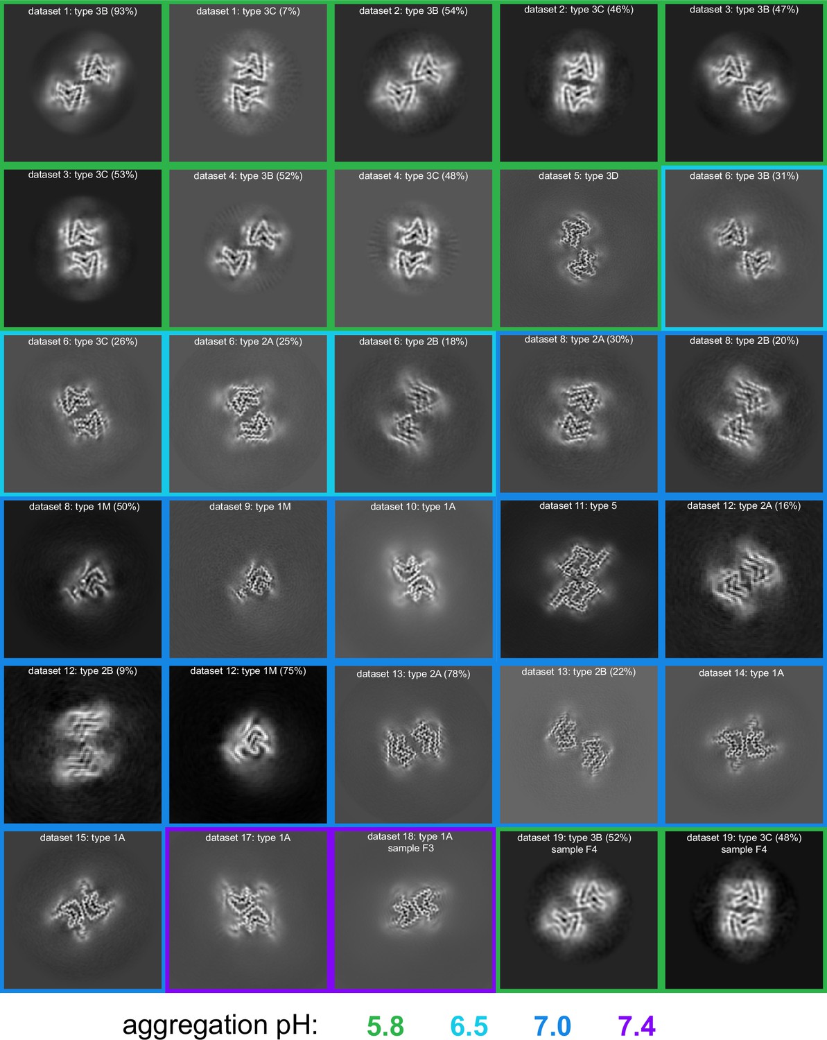
pH-dependence of observed α-synuclein (α-Syn) polymorphs.
An overview of all of the cryo-electron microscopy (cryo-EM)-resolved polymorphs in this study. The images represent a 9.5 Å slice (about two layers of the amyloid) of the 3D map projected in the Z direction. The 3D maps were obtained either from 3D classification or 3D refinement in RELION. The datasets are ordered and numbered as in Table 1. The colored borders indicate the pH at which the fibrils were grown. For datasets from which multiple polymorphs were resolved, the relative percentage of particles corresponding to each polymorph is indicated in parentheses.
Figure 5
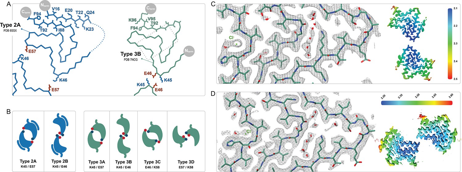
Comparison of the Type 2 and 3 polymorphs.
(A) Protofilaments of polymorphs 2A (blue) and 3B (green) are depicted as Cα traces. The side chains are included on the C-terminal β-strand and the N-terminal segment in the 2A structure in order to highlight the inside-out flipped orientations of their C-terminal β-strands. The dashed box indicates the region highlighted in panels C and D. (B) The two interfaces of Type 2 and the 4 interfaces of Type 3 polymorphs are shown as a cartoon schematic. The charged interfacial residues are indicated by blue/red dots for K/E and listed below each interface. The C-term is indicated as a short tail and Type 2 has the extra N-terminal segment. (C) A close-up view of the Type 3B structure (PDB:8PIC) and (D) Type 3D (E46K) structure (PDB:8PJO) and their EM density, showing the shared set of immobilized water molecules and strong density that has been modeled as a chloride ion. The local resolution maps for each structure are shown to the right with the color scale indicating the resolution range in Å.
Figure 6
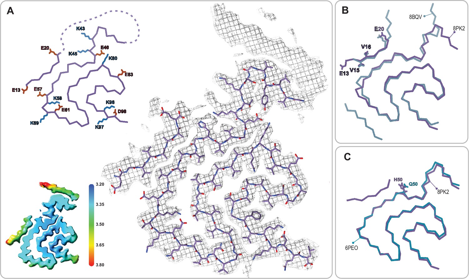
The juvenile-onset synucleinopathy (JOS)-like Type 1M polymorph.
(A) The Type 1M monofilament structure (PDB:8PK2) overlaid with its EM density (including the unmodeled density). The Cα trace is also shown on the left with all K and E side chains indicated as well as the local resolution map for the density with color scale showing the resolution range in Å. (B) An overlay of the Cα trace of the Type 1M and the JOS polymorph (PDB:8BQV) from which the identity of residues 13–20 in the N-terminal strand were assigned. (C) An overlay of the Cα trace of the JOS-like Type 1M to the 1M structure of the H50Q mutant (PDB:6PEO). The structural alignments were done by an LSQ-superposition of residues 51–66.
Figure 7
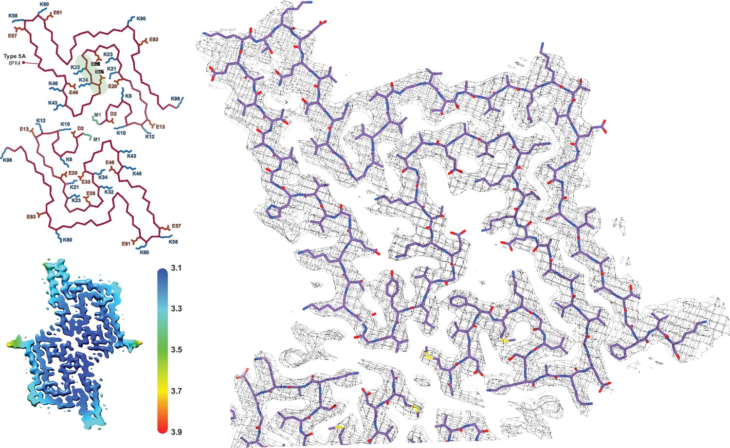
The Type 5 polymorph.
The structure of a Type 5 protofilament (PDB:8PK4) overlaid with its EM density. The Cα trace for the two filaments of the Type 5A fibril is also shown to the left. All of the charged (E/D/K) residues and the acetylated N-terminal Met are labeled and the polar segment that dissects the two cavities is shaded green in the upper chain. The local resolution map is also shown with the color scale indicating the resolution in Å.
Figure 8
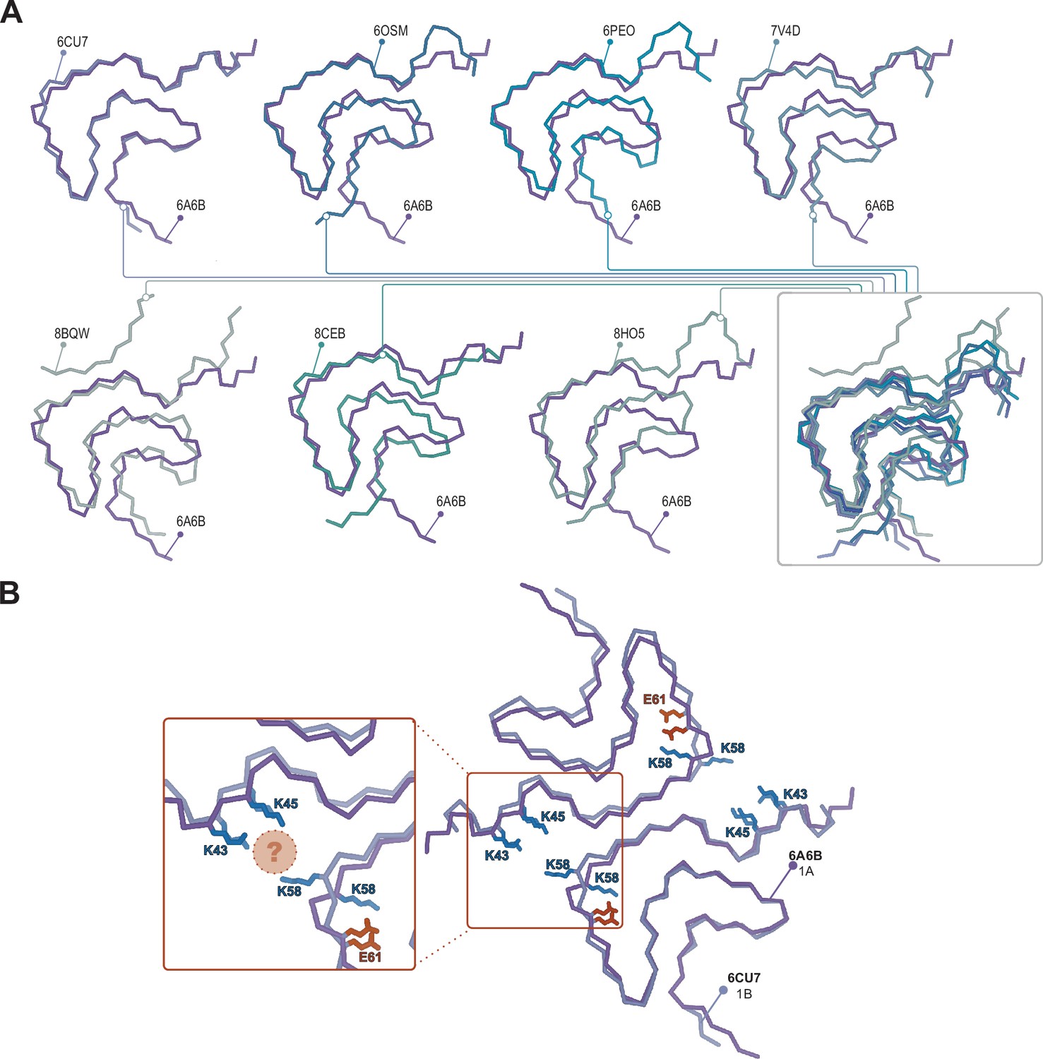
Structural variability within the Type 1 polymorphs.
(A) Seven pairwise overlays of the wild-type 1A structure (PDB:6A6B) with other wild-type and mutant structures depicting the range of structural variability that is found in the Type 1 fold. The structural alignments were done by an LSQ-superposition of the Cα atoms of residues 51–66. The other Type 1 structures from left to right, top to bottom are wild-type 1A without buffer (PDB:6CU7), N-terminally acetylated wild-type 1A residues 1–103 (PDB:6OSM), the H50Q mutant 1M without buffer (PDB:6PEO), wild-type 1A in Tris-buffered saline (PDB:7V4D), the patient-derived juvenile-onset synucleinopathy (JOS) 1M polymorph (PDB:8BQV), mix of wild-type and seven residue JOS-associated insertion mutant 1A in PBS (PDB:8CEB) and N-terminally acetylated wild-type 1M seeded from Parkinson’s disease (PD) patient cerebrospinal fluid (CSF) in PIPES with 500 mM NaCl. (B) Same overlay shown at the top right in A, showing the triad of lysine residues often formed at the interface in the presence of phosphate (PDB:6CU7) compared to the inward-facing orientation of K58 in the absence of phosphate (PDB:6A6B). The location of often observed density, thought to be PO42-, is indicated with the pink sphere.
Figure 9
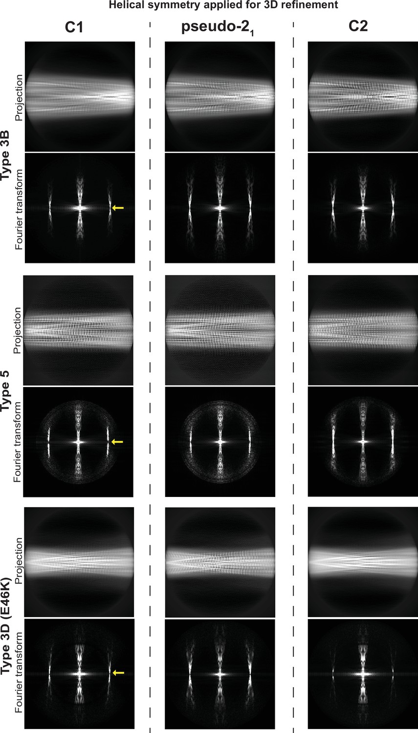
Determination of helical symmetry in Type 3B, 3D, and 5A polymorphs.
2D projections and their Fourier transforms for three different structures (rows) refined with three different types of symmetry (columns). Each of the structures studied was refined as far as possible in a C1 symmetry with a ca. –1° twist and 4.7 Å rise in order to examine the higher order symmetry expected to be present: either C2 with a 4.7 Å rise or a pseudo-21 helical symmetry with ca. –179.5 twist and 2.35 Å rise. A comparison of the projections of the refined volumes indicated that all three of these structures have a pseudo-21 helical symmetry. This can be seen in the C1 projections which lack a mirror symmetry down their middle and in their Fourier transforms which lack an n=0 Bessel function meridional peak in the layer line at 1/4.7 Å (̊location marked with a yellow arrow).
Figure 10
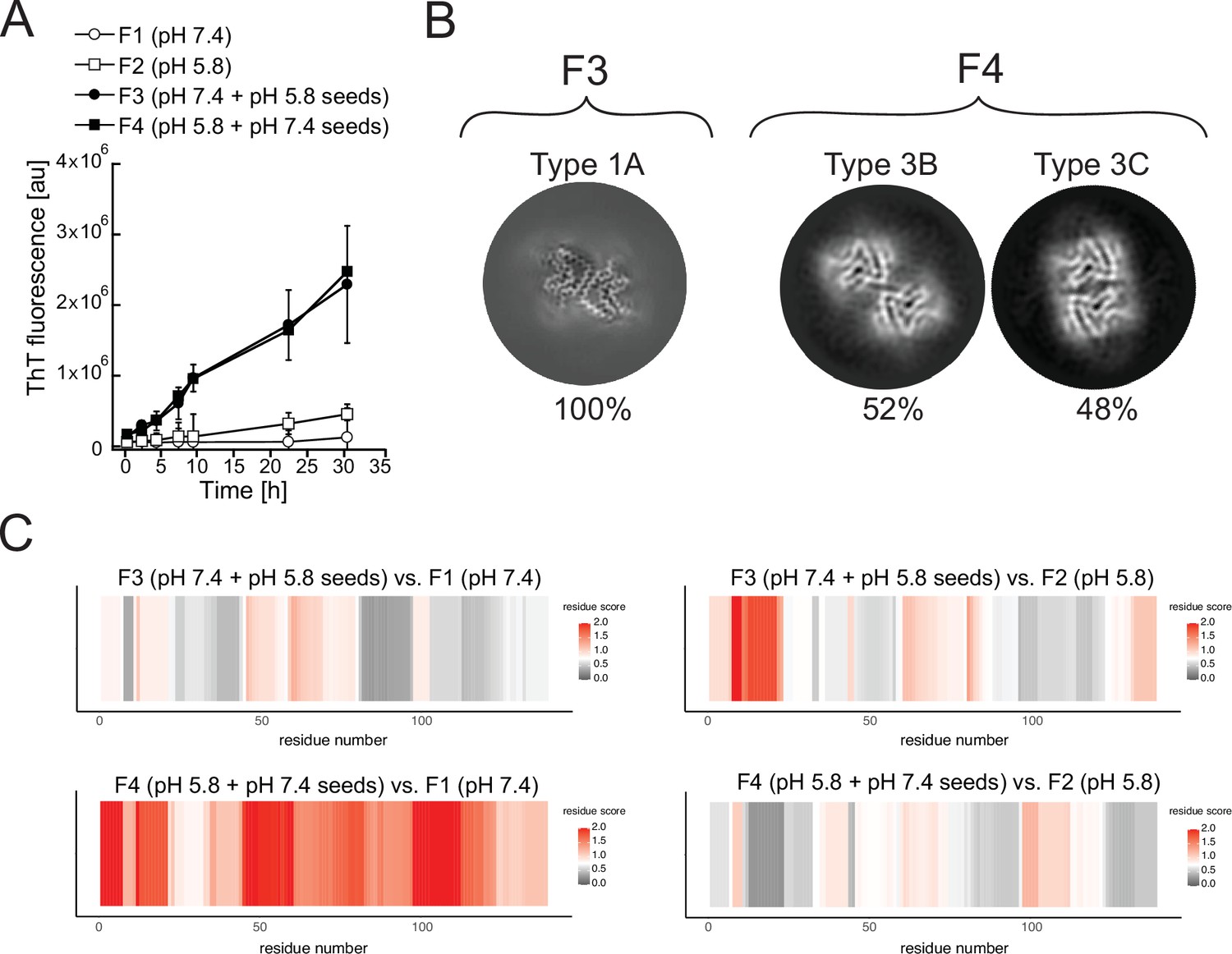
Cross-seeding does not preserve the seed polymorph.
Fibrils produced at pH 7.4 (F1) and pH 5.8 (F2) were used as seeds to generate new fibril samples with fresh α-synuclein monomer: at pH 7.4 with 5% unfragmented pH 5.8 seeds (F3) or at pH 5.8 with pH 7.4 seeds (F4). (A) The effect of cross-seeding with fibrils produced in a different pH from that of the aggregation condition is shown in the aggregations kinetics, as monitored by thioflavin T (ThT) fluorescence. The average values of three independent aggregation measurements are plotted with error bars representing their standard deviations. (B) Cryo-electron microscopy (cryo-EM) analyses of the seeded samples yielded a single 3D class representing polymorph 1A (here depicted as a Z-section) for the F3 fibrils and two classes representing Types 3B and 3C for the F4 fibrils. (C) Limited proteolysis-coupled mass spectrometry (LiP-MS) analysis showing the differences in fibrillar structures in bulk solution. The comparison of seeded fibrils (F3 and F4) with F1 is presented on the left, while the comparison of seeded fibrils with F2 is presented on the right. Differences in structures per residue are plotted along the sequence of α-synuclein in a form of scores (-log10(p-value) × |log2(fold change)|). The more intense the red color, the greater the difference between the two structures in each region. Gray indicates no significant differences, while white indicates the significance threshold corresponding to (-log10(0.05) × |log2(1.5)|).
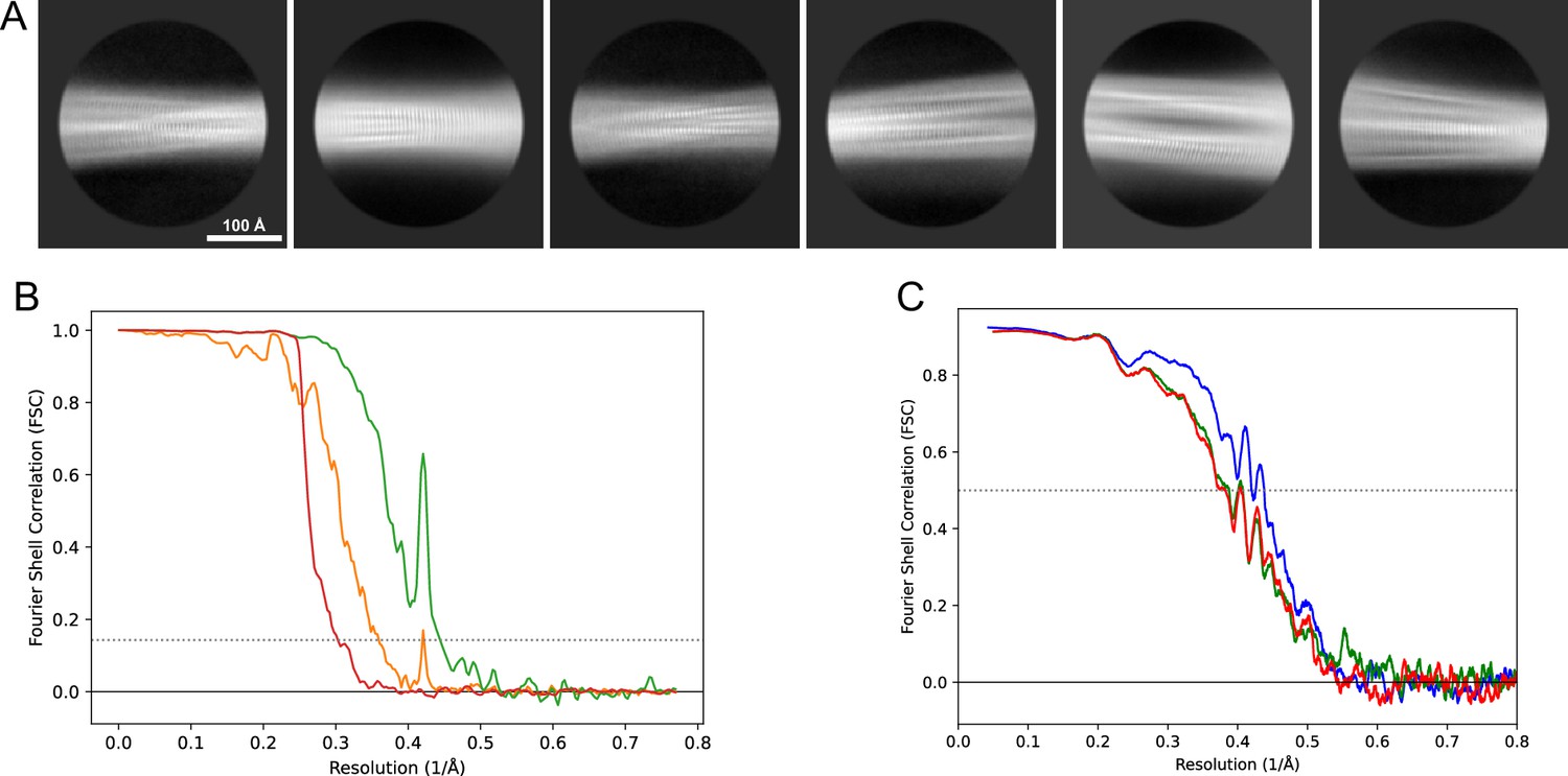
Figure 11
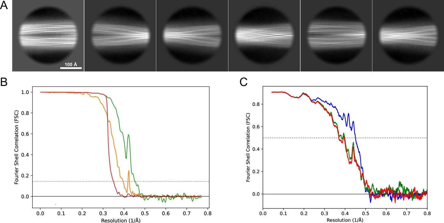
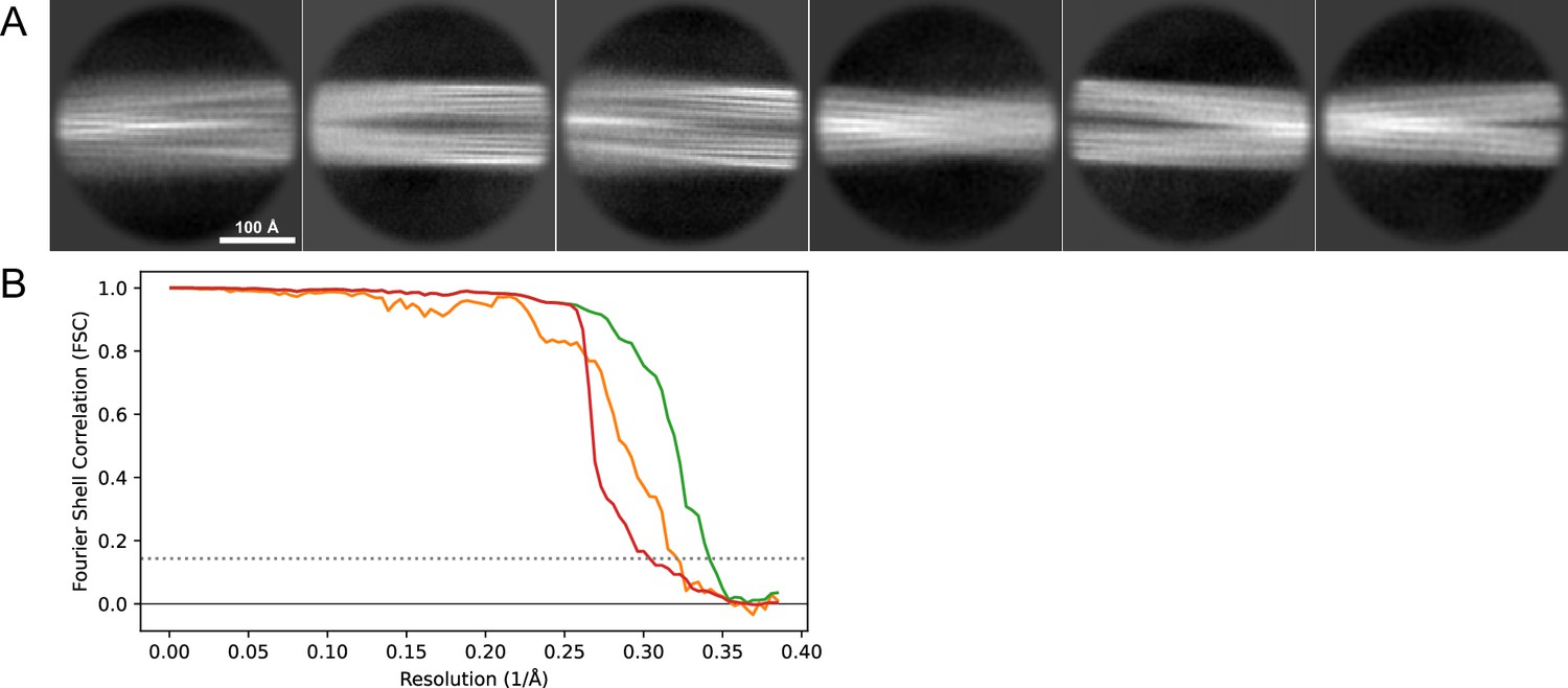
2D classes and half-map and model-map FSC curves for dataset 1, Type 3B.
(A) Representative 2D classes of the segments that were used for the 3D reconstruction. (B) The FSC curves produced during postprocessing in RELION with red showing the plot for the phase randomized, orange the unmasked, and green the masked maps. (C) The model-map FSC curves produced in PHENIX. The blue curve is for the deposited coordinates and full postprocessed map against which it had been fit by real-space refinement in PHENIX. Coordinates were similarly generated by refining against the first half-map and then compared to the same half-map (green) or the second half-map (red).
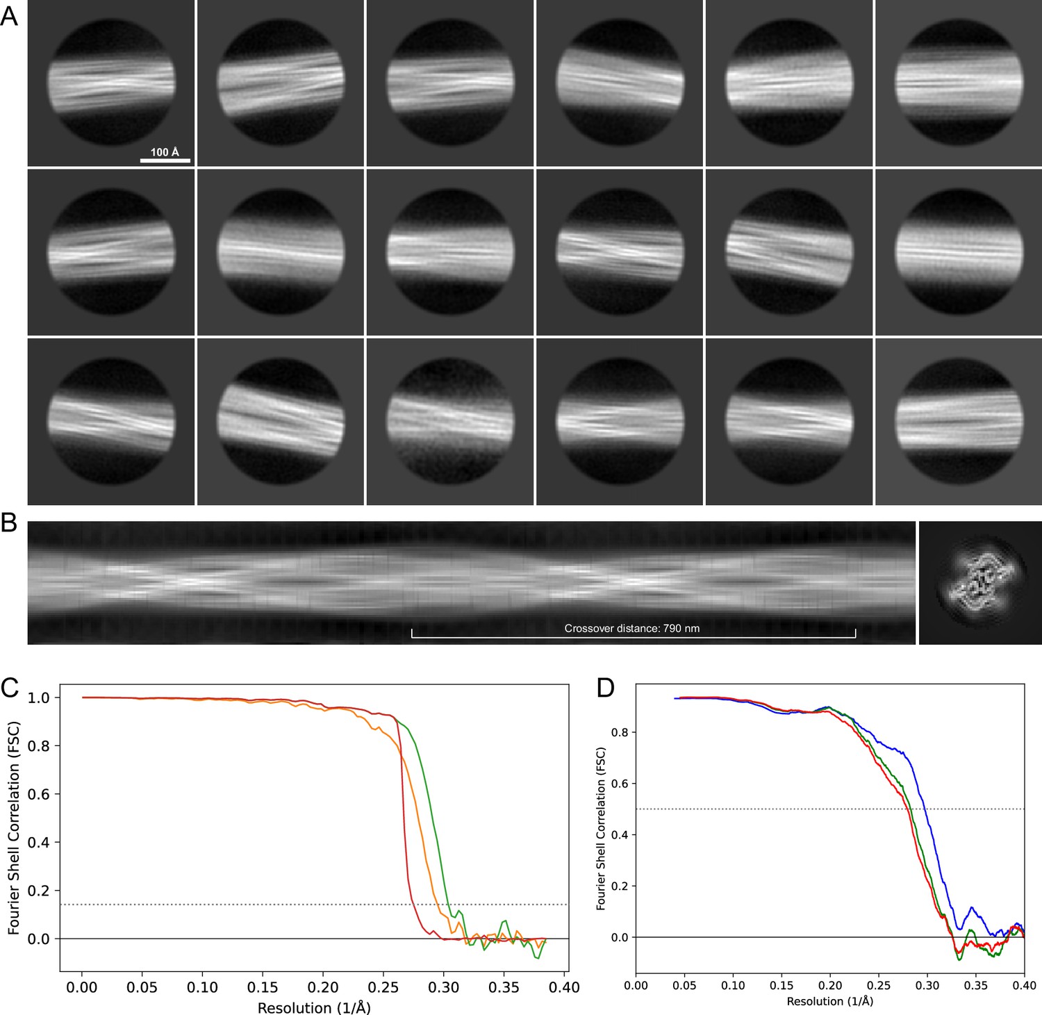
Figure 12
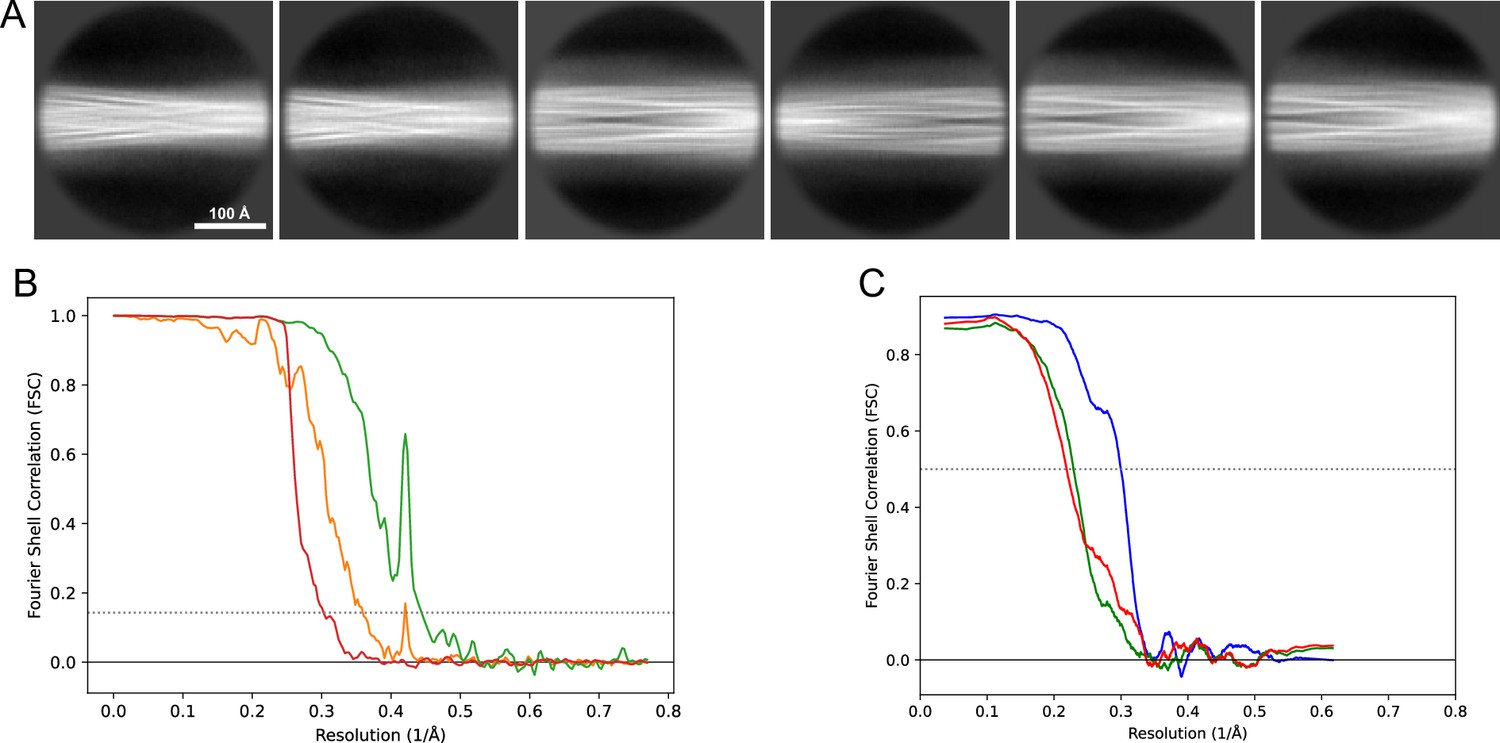
2D classes and half-map and model-map FSC curves for dataset 3, Type 3C.
(A) Representative 2D classes of the segments that were used for the 3D reconstruction. (B) The FSC curves produced during postprocessing in RELION with red showing the plot for the phase randomized, orange the unmasked, and green the masked maps. (C) The model-map FSC curves produced in PHENIX. The blue curve is for the deposited coordinates and full postprocessed map against which it had been fit by real-space refinement in PHENIX. Coordinates were similarly generated by refining against the first half-map and then compared to the same half-map (green) or the second half-map (red).
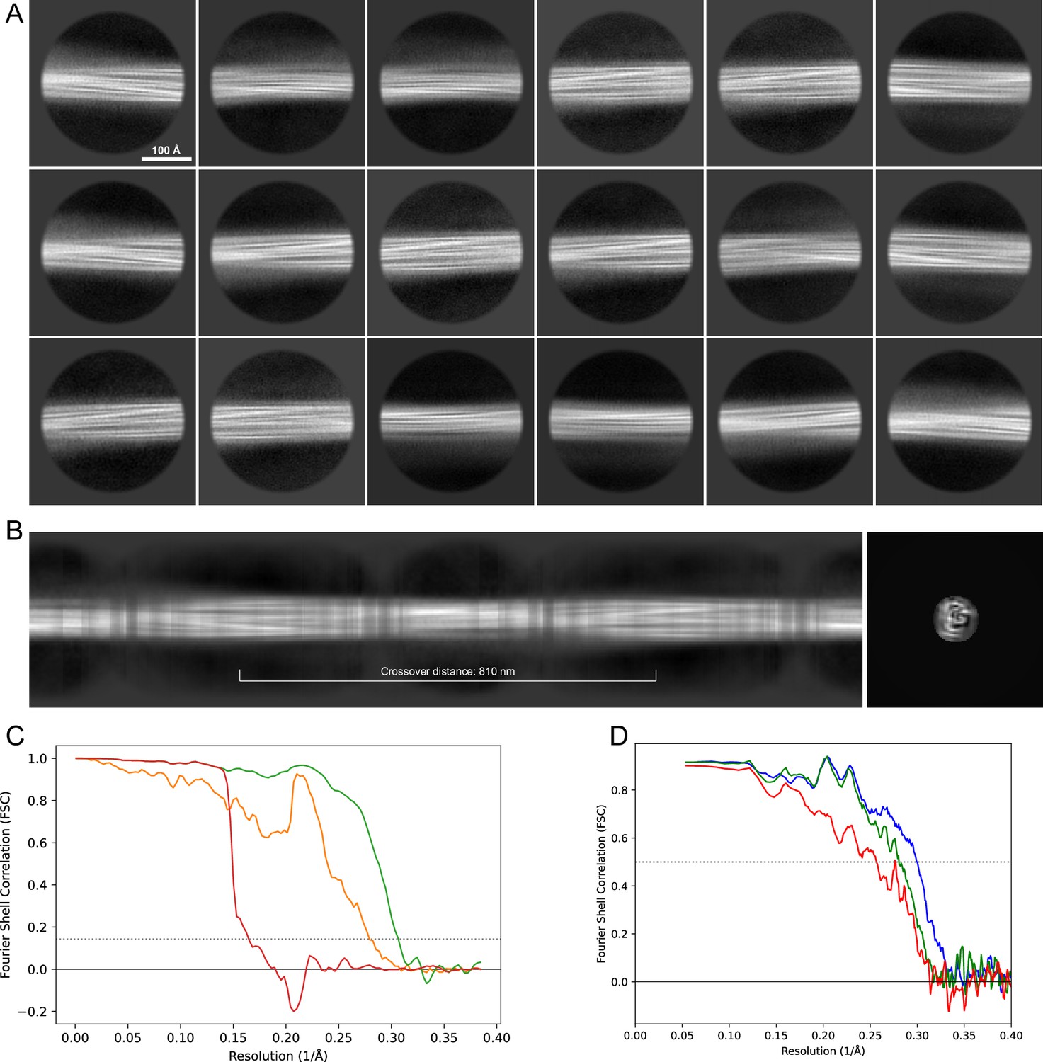
Figure 13
2D classes and half-map and model-map FSC curves for dataset 5, Type 3D.
(A) Representative 2D classes of the segments that were used for the 3D reconstruction. (B) The FSC curves produced during postprocessing in RELION with red showing the plot for the phase randomized, orange the unmasked, and green the masked maps. (C) The model-map FSC curves produced in PHENIX. The blue curve is for the deposited coordinates and full postprocessed map against which it had been fit by real-space refinement in PHENIX. Coordinates were similarly generated by refining against the first half-map and then compared to the same half-map (green) or the second half-map (red).
Figure 14
2D classes and half-map and model-map FSC curves for dataset 8, Type 5.
(A) The 2D classes of the segments that were used to produce the initial model in relion_helix_inimodel2d. (B) The output of relion_helix_inimodel2d shown as the summed 2D classes and a Z-projection of the reconstructed 3D model used as input for refinement in the 3D refinement. (C) The FSC curves produced during postprocessing in RELION with red showing the plot for the phase randomized, orange the unmasked, and green the masked 2D classes and half-map FSC curves for dataset 13, Type 2A.maps. (D) The model-map FSC curves produced in PHENIX. The blue curve is for the deposited coordinates and full postprocessed map against which it had been fit by real-space refinement in PHENIX. Coordinates were similarly generated by refining against the first half-map and then compared to the same half-map (green) or the second half-map (red).
Figure 15
2D classes and half-map and model-map FSC curves for dataset 9, Type 1M.
(A) The 2D classes of the segments that were used to produce the initial model in relion_helix_inimodel2d. (B) The output of relion_helix_inimodel2d shown as the summed 2D classes and a Z-projection of the reconstructed 3D model used as input for refinement in the 3D refinement. (C) The FSC curves produced during postprocessing in RELION with red showing the plot for the phase randomized, orange the unmasked, and green the masked maps. (D) The model-map FSC curves produced in PHENIX. The blue curve is for the deposited coordinates and full postprocessed map against which it had been fit by real-space refinement in PHENIX. Coordinates were similarly generated by refining against the first half-map and then compared to the same half-map (green) or the second half-map (red).
Figure 16
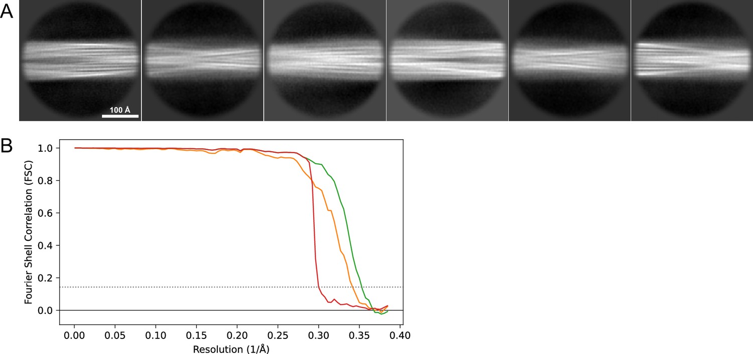
2D classes and half-map FSC curves for dataset 13, Type 2A.
(A) Representative 2D classes of the segments that were used for the 3D reconstruction. (B) The FSC curves produced during postprocessing in RELION with red showing the plot for the phase randomized, orange the unmasked, and green the masked maps.
Figure 17
2D classes and half-map FSC curves for dataset 13, Type 2B.
(A) Representative 2D classes of the segments that were used for the 3D reconstruction. (B) The FSC curves produced during postprocessing in RELION with red showing the plot for the phase randomized, orange the unmasked, and green the masked maps.
Tables
Table 1
Cryo-electron microscopy (cryo-EM) samples analyzed for this manuscript.
| Dataset | Construct | Batch | Aggregation condition | pH ‡ | Polymorph(s) | Relative abundance§ | Refinement stage |
|---|---|---|---|---|---|---|---|
| 1 | Ac-1–140* | 2 | PBS† | 5.8 | 3B¶:3C | 93%:7% | 3B, see Tables 2 : 3C, 3D classification |
| 2 | Ac-1–140 | 6 | PBS | 5.8 | 3B:3C | 54%:46% | 3D classification |
| 3 | Ac-1–140 | 3 | PBS+50 mM NaCl | 5.8 | 3B:3C | 47%:53% | 3C, see Table 2 : 3B, 3D classification |
| 4 | Ac-1–140 | 4 | PBS+100 mM NaCl | 5.8 | 3B:3C | 52%:48% | 3D classification |
| Ac-1–140 (E46K) | PBS+50 mM NaCl | 5.8 | 3D | See Table 2 | |||
| 6 | Ac-1–140 | 7 | PBS | 6.5 | 2A:2B:3B:3C | 25%:18%:31%:26% | Filament subset selection followed by 3D refinement to 3.51 Å, 4.73 Å, 4.56 Å, 4.06 Å respectively |
| 7 | Ac-1–140 | 4 | 20 mM Tris, 140 mM NaCl | 7.0 | 1A | 3D refinement 3.65 Å | |
| 8 | Ac-1–140 | 4 | PBS | 7.0 | 5A | See Table 2 | |
| 9 | Ac-1–140 | 5 | PBS | 7.0 | 1M | See Table 2 | |
| 10 | Ac-1–140 | 5 | PBS | 7.0 | Non-twisted** | ||
| 11 | Ac-1–140 | 7 | PBS | 7.0 | 2A:2B:1M | 30%:20%:50%‡ ‡ | Filament subset selection followed by 3D refinement to 4.2 Å, 4.9 Å and 4.8 Å respectively |
| 12 | Ac-1–140 | 7 | PBS | 7.0 | 2A:2B:1M | 16%:9%:75%‡ ‡ | Filament subset selection followed by 3D refinement to 5.4 Å, 6.4 Å and 5.8 Å respectively†† |
| 13 | Ac-1–140 | 8 | PBS | 7.0 | 2A:2B | 78%:22% | Filament subset selection - see Table 2†† |
| 14 | Ac-1–140 | 8 | PBS | 7.0 | 1A | 3D refinement to 2.95 Å | |
| 15 | Ac-1–140 | 8 | PBS | 7.0 | 1A | 3D refinement to 3.94 Å | |
| 16 | Ac-1–140 | 8 | PBS | 7.0 | Non-twisted and clumped** | ||
| 17 | Ac-1–140 | 4 | PBS | 7.4 | 1A | 3D refinement to 3.73 Å | |
| 18 (F3) | Ac-1–140 | 5 | PBS +5% pH 5.8 seeds | 7.4 | 1A | 3D refinement to 3.50 Å | |
| 19 (F4) | Ac-1–140 | 7 | PBS +5% pH 7.4 seeds | 5.8 | 3B:3C | 52%:48% | 3D classification |
-
*
All constructs are full-length, N-terminally acetylated (Ac).
-
†
PBS is a 10 mM phosphate buffer solution with 137 mM NaCl and 2.7 mM KCl.
-
‡
The pH was adjusted after dissolving the PBS tablet (Sigma-Aldrich) by the addition of HCl.
-
§
In samples for which more than one polymorph could be identified by 3D classification or filament subset selection in RELION.
-
¶
Underlining indicates data that was used for 3D refinement of the deposited maps and for building the deposited coordinates.
-
**
This data could not be analyzed by helical reconstruction as only non-twisted fibrils were present.
-
††
Filament subset selection was run after 2D classification of the entire set of auto-picked particles. The identified filament classes were individually 2D classified and these classes used to create an initial model with relion_helix_inimodel2d which was used for automated 3D refinement. In the case of dataset 13 followed by CTF refinement and Bayesian polishing in RELION.
-
‡ ‡
Due to the small size of these datasets, the relative abundances are not likely to be precise.
Table 2
Cryo-electron microscopy (cryo-EM) structure determination statistics.
| Polymorph | 1M | 2A | 2B | 3B | 3C | 5A | 3D (E46K) |
|---|---|---|---|---|---|---|---|
| Data collection | |||||||
| Pixel size [Å] | 0.65 | 0.65 | 0.65 | 0.65 | 0.65 | 0.65 | 0.65 |
| Defocus range [µm] | –0.8 to –2.5 | 0.8 to –2.5 | 0.8 to –2.5 | –0.8 to –2.5 | –0.8 to –2.5 | –0.8 to –2.5 | –0.8 to –2.5 |
| Voltage [kV] | 300 | 300 | 300 | 300 | 300 | 300 | 300 |
| Number of frames | 40 | 40 | 40 | 40 | 40 | 40 | 40 |
| Total dose [e-/Å2] | 69 | 58.5 | 58.5 | 62 | 67 | 75 | 65 |
| Reconstruction | |||||||
| Reconstruction box width [pixels] | 256 | 200 | 200 | 512 | 256 | 256 | 512 |
| Inter-box distance [Å] | 33 | 33 | 33 | 33 | 33 | 33 | 33 |
| Reconstruction pixel size [Å] | 1.3 | 1.3 | 1.3 | 0.65 | 1.3 | 1.3 | 0.65 |
| Micrographs | 1,624 | 1339 | 1339 | 7,729 | 3,127 | 1,850 | 4,666 |
| Initially extracted segments | 84,666 | 238,570 | 238,570 | 279,929 | 159,308 | 109,817 | 287,018 |
| Segments after 2D and 3D classification | 19,800 | 91,238 | 26,426 | 178,710 | 28,022 | 86,219 | 40,181 |
| 3D refinement resolution [Å] (FSC>0.143) | 3.58 | 2.99 | 3.13 | 2.64 | 3.41 | 3.40 | 2.40 |
| Final resolution [Å] (FSC >0.143) | 3.26 | 2.86 | 2.95 | 2.23 | 3.41 | 3.30 | 2.31 |
| Estimated map sharpening B-factor [Å2] | –43.8 | –73.0 | –74.9 | –51.7 | –101.7 | –87.4 | –32.8 |
| Axial symmetry | C1 | C2 | C1 | C1 | C2 | C1 | C1 |
| Helical rise [Å] | 4.79 | 4.82 | 2.39 | 2.37 | 4.77 | 2.42 | 2.41 |
| Helical twist [°] | –0.95 | –0.80 | 179.6 | 179.5 | –0.995 | 179.6 | 179.5 |
| Model composition and validation | |||||||
| Non-hydrogen atoms (5 layers) | 2515 | – | – | 4550 | 4500 | 6690 | 4450 |
| Protein residues (5 layers) | 365 | – | – | 640 | 650 | 960 | 630 |
| R.m.s. deviations bond length [Å] | 0.008 | – | – | 0.005 | 0.007 | 0.006 | 0.007 |
| R.m.s. deviations bond angles [°] | 1.166 | – | – | 0.637 | 0.976 | 0.863 | 1.093 |
| MolProbity score | 1.66 | – | – | 2.01 | 1.33 | 1.64 | 1.60 |
| Clashscore | 3.71 | – | – | 7.42 | 1.62 | 4.72 | 3.57 |
| Rotamer outliers [%] | 0 | – | – | 2.22 | 1.3 | 0 | 0.68 |
| Ramachandran plot favored [%] | 91.6 | – | – | 95.2 | 95.2 | 94.2 | 92.8 |
| Ramachandran plot allowed [%] | 81.4 | – | – | 4.8 | 4.8 | 5.8 | 7.2 |
| Ramachandran plot disallowed [%] | 0 | – | – | 0 | 0 | 0 | 0 |
| Model resolution [Å] (FSC >0.143/0.5) | 3.1/3.3 | – | – | 2.0/2.2 | 3.1/3.3 | 3.1/3.4 | 2.0/2.4 |
| PDB code | 8PK2 | – | – | 9FYP | 8PIX | 8PK4 | 8PJO |
| EMDB-ID | 17723 | 50860 | 50077 | 50888 | 17693 | 17726 | 17714 |
Additional files
Download links
A two-part list of links to download the article, or parts of the article, in various formats.
Downloads (link to download the article as PDF)
Open citations (links to open the citations from this article in various online reference manager services)
Cite this article (links to download the citations from this article in formats compatible with various reference manager tools)
On the pH-dependence of α-synuclein amyloid polymorphism and the role of secondary nucleation in seed-based amyloid propagation
eLife 12:RP93562.
https://doi.org/10.7554/eLife.93562.4


